ODE Integrators I: Explicit Methods

Ordinary differential equations form the mathematical foundation of physics. They describe how systems evolve in time, e.g., Newton’s second law of motion is

\begin{align} f = m a = m \frac{d^2x}{dt^2}, \end{align}

(1)

which is a second-order ODE relating force to acceleration. More generally, an ODE relates a function of time to its time derivatives.

While ODEs capture the essence of dynamics, analytic solutions are possible only in special cases. Most real systems involve nonlinear forces, damping, or external driving terms that make exact solutions impossible. Numerical integration allows us to approximate trajectories step by step and study systems far beyond what can be solved by hand.

Problem Definition and Types of ODEs¶

Consider two forms of first-order ODEs:

Time-dependent forcing only:
$\begin{align} \frac{dx}{dt} = f(t). \end{align}$
(2)
Here, the derivative depends only on time. Solutions are obtained by direct integration:
$\begin{align} x(t) = x(t_0) + \int_{t_0}^{t} f(t') \, dt'. \end{align}$
(3)
State- and time-dependent dynamics:
$\begin{align} \frac{dx}{dt} = f(x, t). \end{align}$
(4)
Now, the derivative depends on the state $x$ itself. The function we want to solve for also appears inside the RHS, making direct integration impossible. We cannot evaluate the integral without already knowing $x(t)$ at intermediate points.

The first type reduces to standard numerical quadrature (trapezoidal rule, Simpson’s rule, etc.), which we studied earlier. The second case, nonlinear dependence on both $x$ and $t$ , is the typical situation in physics. Examples include planetary orbits, nonlinear oscillators, chaotic systems, and interacting biological populations. In such cases:

Direct integration is often not feasible, the problem must be solved as an initial value problem (IVP).
Analytic solutions are often unknown or intractable.
Numerical methods approximate the solution incrementally, using small time steps to trace the system’s evolution.

By discretizing time and advancing step-by-step, we can model the behavior of even the most complex systems. This is the core idea behind numerical ODE integrators.

Forward Euler Method¶

Euler’s method is the simplest techniques for numerically solving ordinary differential equations. This method provides an easy way to approximate the solution of an IVP by advancing one small step at a time.

We can apply Euler’s method to an ODE of the form:

\begin{align} \frac{dx}{dt} = f(x, t), \quad x(t_0) = x_0 \end{align}

(5)

where $x_0$ is the initial value of $x$ at time $t = t_0$ . However, as we will see below, it is usually not recommanded in pratical calculations because of its stability properties.

There are three simple ways to derive Euler’s method. The easiest way is simply hold $x$ fixed in $f(x, t)$ and apply the left Reimann sum. The left Reimann sum is first order in step size by approximating $f(x, t)$ as a constant. In this sense, holding $x$ is somewhat “self-consistent” in terms of approximation order.

We then recall the definition of a deriviative:

\begin{align} f(x, t) = \frac{dx}{dt} = \lim_{\Delta t\rightarrow 0}\frac{x(t + \Delta t) - x(t)}{\Delta t}. \end{align}

(6)

If we simply remove the limit and keep the “finite difference” part, then it is trivial to show

\begin{align} x(t + \Delta t) &\approx x(t) + f(x(t), t)\Delta t. \end{align}

(7)

Which is nothing but again the forward Euler method. While very intuitive, the above two derivations do not formally show the order of the Euler method.

We may also consider a numerical approximation to the solution of an ODE. We approximate the solution at time $t_{n+1} = t_n + \Delta t$ by using the Taylor expansion:

\begin{align} x(t_{n+1}) = x(t_n) + f(x(t_n), t_n) \Delta t + \mathcal{O}(\Delta t^2) \end{align}

(8)

Neglecting the higher-order terms in the expansion, we obtain once again the Forward Euler Method:

\begin{align} x_{n+1} = x_n + f(x_n, t_n) \Delta t \end{align}

(9)

It is thus a step-by-step approach that proceeds by evaluating $f(x, t)$ at each time point and then advancing to the next point. It is an explicit method in 1st order.

Let’s solve the simple differential equation:

\begin{align} \frac{dx}{dt} = \lambda x(t) \end{align}

(10)

This equation has solution

\begin{align} x(t) = \exp[\lambda(t-t_0)] \end{align}

(11)

If we choose $\lambda = 1$ and $x(0) = 1$ , the solutoin reduces to $x(t) = \exp(t)$ .

# Let's visualize the solution:

import numpy as np
from matplotlib import pyplot as plt

T = np.linspace(0, 1, 1001)
X = np.exp(T)

plt.plot(T, X, label=r"$\exp(t)$")
plt.xlabel(r"$t$")
plt.ylabel(r"$x(t)$")
plt.legend()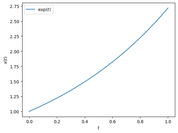

# Let's implement Euler's method, with history

def Euler(f, x, t, dt, n):
    X = [np.array(x)]
    T = [np.array(t)]
    for _ in range(n):
        X.append(X[-1] + dt * f(X[-1]))
        T.append(T[-1] + dt)
    return np.array(X), np.array(T)

# Let's test Euler's method

f  = lambda x: x

n  = 10
dt = 1/n

x0 = 1
t0 = 0

X1, T1 = Euler(f, x0, t0, dt, n)

plt.plot(T,  X,        label=r"$\exp(t)$")
plt.plot(T1, X1, "o-", label=r"Forward Euler")
plt.xlabel(r"$t$")
plt.ylabel(r"$x(t)$")
plt.legend()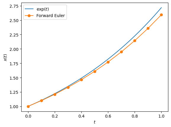

# As always, we can study the convergence of the numerical method

def Err(n=100):
    X1, T1 = Euler(f, 1, 0, 1/n, n)
    X = np.exp(T1)
    return np.max(abs(X1 - X))

N  = np.array([32, 64, 128, 256, 512, 1024])
E1 = np.array([Err(n) for n in N])

plt.loglog(N, 1/N, "k--", label=r"1/n")
plt.loglog(N, E1,  "o:",  label=r"Forward Euler")
plt.xlabel(r"$n$")
plt.ylabel(r"$\text{err} = \max|x_\text{numeric} - x|$")
plt.legend()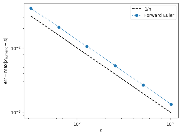

High-Order and System of ODEs¶

In computational astrophysics, we often encounter systems governed by Newton’s laws:

\begin{align} m \frac{d^2 x}{dt^2} = f(x, t) \end{align}

(12)

This equation is a second-order ordinary differential equation because it involves the second derivative of $x$ with respect to $t$ . However, it is often more practical to convert second-order ODEs into a system of first-order ODEs. To do this, we introduce a new variable, $v = dx/dt$ , representing the velocity of the object. This substitution allows us to rewrite the second-order ODE as two coupled first-order ODEs:

\begin{align} \frac{dx}{dt} &= v \\ \frac{dv}{dt} &= \frac{1}{m}f(x, t) \end{align}

(13)

This formulation provides a convenient way for numerical methods, which are generally well-suited to solving systems of first-order ODEs. To further simplify, we can express these equations in vector notation by defining $\mathbf{x} = [x, v]^t$ and $\mathbf{f} = [v, f/m]^t$ . The system then becomes:

\begin{align} \frac{d\mathbf{x}}{dt} = \mathbf{f}(\mathbf{x}, t). \end{align}

(14)

This vector form emphasizes the structure of the system and enables us to apply general numerical techniques to solve both equations simultaneously.

To illustrate this approach, let’s consider a classic example: the simple pendulum under gravity. The motion of a pendulum of length $l$ , swinging under gravity $g$ , can be described by the second-order equation:

\begin{align} \frac{d^2\theta}{dt^2} + \frac{g}{l} \sin\theta = 0 \end{align}

(15)

Here, $\theta(t)$ is the angle of the pendulum with the vertical, and the term $\sin \theta$ introduces nonlinearity, which makes the equation challenging to solve analytically. Converting this equation into a system of first-order ODEs allows us to handle it more effectively with numerical methods. We define $\Omega = \frac{d\theta}{dt}$ , the angular velocity, leading to the following system:

\begin{align} \frac{d\theta(t)}{dt} &= \Omega(t)\\ \frac{d\Omega(t)}{dt} &= - \frac{g}{l}\sin\theta(t) \end{align}

(16)

In vector notation, we represent the system as:

\begin{align} \frac{d\mathbf{x}(t)}{dt} = \mathbf{f}(\mathbf{x}, t) \end{align}

(17)

where

\begin{align} \mathbf{x} &= \begin{bmatrix} \theta(t) \\ \Omega(t) \end{bmatrix}, \\ \mathbf{f}(\mathbf{x}, t) &= \begin{bmatrix} \Omega(t) \\ -\frac{g}{l} \sin \theta(t) \end{bmatrix}. \end{align}

(18)

In later part of the lecture, we will try to solve this full problem. But to derive and compare different numerical methods, let’s first reduce the problem to something that has analytical solutions. Specifically, we can simplify the pendulum problem further by assuming small oscillations, where the angle $\theta$ is small enough that $\sin \theta \approx \theta$ . This approximation linearizes the equation of motion, reducing the system to a simple harmonic oscillator.

In this approximation, the equation of motion becomes:

\begin{align} \frac{d^2 \theta}{dt^2} + \frac{g}{l} \theta = 0 \end{align}

(19)

As a result, the system of ODEs becomes:

\begin{align} \mathbf{x} &= \begin{bmatrix} \theta(t) \\ \Omega(t) \end{bmatrix}, \\ \mathbf{f}(\mathbf{x}, t) &= \begin{bmatrix} \Omega(t) \\ -\frac{g}{l} \theta(t) \end{bmatrix}. \end{align}

(20)

# Let's first plot the analytical solution

T     = np.linspace(0, 10, 101)
Theta = 0.01 * np.sin(T)

plt.plot(T, Theta, label=r"$0.01\sin(t)$")
plt.xlabel(r"$t$")
plt.ylabel(r"$\theta(t)$")
plt.legend()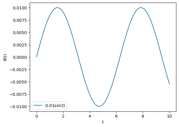

# Thanks to operator overriding, our forward Euler method is almost
# ready to solve system of ODEs!
# There is no need to rewrite it!

# Compare the analytical and numerical solutions

def F(x):
    theta, omega = x
    return np.array([omega, -theta])

n  = 64
dt = 10 / n

X0 = [0, 0.01]
t0 = 0

X1, T1 = Euler(F, X0, t0, dt, n)

Theta1 = X1[:,0]
Omega1 = X1[:,1]

plt.plot(T,  Theta,        label=r"$0.01\sin(t)$")
plt.plot(T1, Theta1, "o-", label=r"Forward Euler")
plt.xlabel(r"$t$")
plt.ylabel(r"$\theta(t)$")
plt.legend()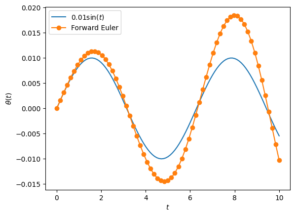

# Again, we can study the convergence of the numerical method

def Err(integrator, n=100):
    Xf, Tf = integrator(F, [0, 0.01], 0, 10/n, n)
    Thetaf = Xf[:,0]
    Theta  = 0.01 * np.sin(Tf)
    return np.max(abs(Thetaf - Theta))

N  = np.array([64, 128, 256, 512, 1024])
E1 = np.array([Err(Euler, n) for n in N])

plt.loglog(N, 1/N, "k--", label=r"$1/n$")
plt.loglog(N, E1,  "o:",  label=r"Forward Euler")
plt.xlabel(r"$n$")
plt.ylabel(r"$\text{err} = \max|x_\text{numeric} - x|$")
plt.legend()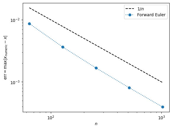

Second-Order Runge-Kutta Method¶

The Forward Euler method is only first-order accurate, meaning its error decreases linearly with the step size $\Delta t$ , as we saw in the convergence plots. While it is simple to implement, this method’s convergence rate is too slow. Achieving higher accuracy requires very small steps, which can become computationally expensive.

This naturally raises the question: can we improve the convergence rate of our numerical solution, reducing the error more rapidly as we use smaller steps?

To explore this, we can draw inspiration from our previous work on numerical integration. In that context, we observed that the midpoint (or central) Riemann sum converges faster than the left or right Riemann sums. This suggests that a midpoint approach may also provide advantages in solving ODEs.

One possible improvement is to propose a midpoint method that attempts to evaluate the function $\mathbf{f}$ at the midpoint between steps. Mathematically, this approach can be expressed as:

\begin{align} \mathbf{x}_{n+1} = \mathbf{x}_n + \mathbf{f}(\mathbf{x}_{n+1/2}, t_{n+1/2}) \Delta t \end{align}

(21)

However, a significant problem arises: the midpoint value $\mathbf{f}_{n+1/2} \equiv \mathbf{f}(\mathbf{x}_{n+1/2}, t_{n+1/2})$ is unknown at step $n$ . We need to know the value of $\mathbf{x}$ at the midpoint $t_{n+1/2}$ to use this method, but this value cannot be calculated without already knowing the future values of $\mathbf{x}$ . This issue makes a straightforward midpoint method impractical for generic ODEs, where $\mathbf{f}$ depends on both $\mathbf{x}$ and $t$ .

An exception occurs if $\mathbf{f}$ depends only on $t$ , as in $d\mathbf{x}/dt = \mathbf{f}(t)$ ; in such cases, a true midpoint method is feasible, which is nothing but out middle Reimann sum. However, for most ODEs, including those where $\mathbf{f}$ depends on $\mathbf{f}$ , a different approach is necessary.

To work around this issue, we can approximate the midpoint value instead of calculating it exactly. It suffices to find an approximate solution for $\mathbf{x}$ at the half-step, which we denote as $\mathbf{x}_{n+1/2}$ .

The simplest way to do this is to use the Forward Euler method to compute an estimated value at the midpoint. Specifically, we can approximate $\mathbf{x}$ at $t_{n+1/2}$ as:

\begin{align} \tilde{\mathbf{x}}_{n+1/2} = \mathbf{x}_n + \mathbf{f}(\mathbf{x}_n, t_n) \frac{\Delta t}{2} \end{align}

(22)

Using this half-step approximation, we then proceed with a full step to find $\mathbf{x}_{n+1}$ by evaluating $f$ at the midpoint:

\begin{align} \mathbf{x}_{n+1} = \mathbf{x}_n + f(\tilde{\mathbf{x}}_{n+1/2}, t_{n+1/2}) \Delta t \end{align}

(23)

This approach, known as the second-order Runge-Kutta method, incorporates midpoint information and achieves second-order accuracy.

This second-order Runge-Kutta method improves convergence by leveraging an approximate midpoint, resulting in a more accurate solution than the first-order Euler method without prohibitively small step size.

def RK2(f, x, t, dt, n):
    X = [np.array(x)]
    T = [np.array(t)]
    for _ in range(n):
        k1 = f(X[-1])
        k2 = f(X[-1] + 0.5 * dt * k1)
        X.append(X[-1] + dt * k2)
        T.append(T[-1] + dt)
    return np.array(X), np.array(T)

n  = 32
dt = 10 / n
X0 = [0, 0.01]
t0 = 0

X2, T2 = RK2(F, X0, 0, dt, n)
plt.plot(T,  0.01 * np.sin(T), label=r"$0.01\sin(t)$")
plt.plot(T2, X2[:,0], "o-",    label=r"RK2")
plt.xlabel(r"$t$")
plt.ylabel(r"$\theta(t)$")
plt.legend()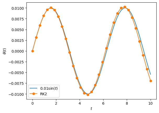

X1, T1 = Euler(F, X0, 0, dt/2, 2*n)
plt.plot(T,       0.01 * np.sin(T),            label=r"$0.01\sin(t)$")
plt.plot(T2,      X2[:,0],   'o-',             label=r"RK2")
plt.plot(T1[::2], X1[::2,0], 'o-', mfc='none', label=r"Substep Forward Euler")
plt.plot(T1,      X1[:,0],   '.',              label=r"Substeps")
plt.xlabel(r"$t$")
plt.ylabel(r"$\theta(t)$")
plt.legend()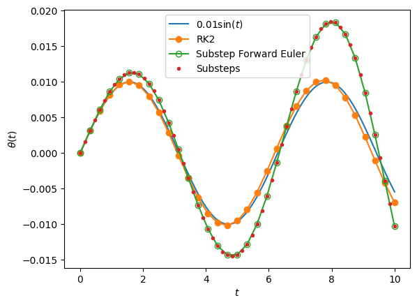

# Again, we can study the convergence of the numerical method

N   = np.array([32, 64, 128, 256, 512, 1024])
E1  = np.array([Err(Euler, n) for n in   N])
E12 = np.array([Err(Euler, n) for n in 2*N])
E2  = np.array([Err(RK2,   n) for n in   N])

plt.loglog(N, 1/N,    "k--", label=r"$1/n$")
plt.loglog(N, 1/N**2, "k-.", label=r"$1/n^2$")
plt.loglog(N, E1,     "o:",  label=r"Forward Euler")
plt.loglog(N, E12,    "o-",  label=r"Substep Euler")
plt.loglog(N, E2,     "o-",  label=r"RK2")
plt.xlabel(r"$n$")
plt.ylabel(r"$\text{err} = \max|x_\text{numeric} - x|$")
plt.legend()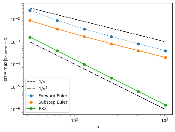

The convergence plot clearly demonstrates that RK2 achieves second-order accuracy. This means that the error decreases quadratically with the step size $\Delta t$ . For example, using 1024 points for the integration not only doubles the computational cost compared to using 512 points but also improves the accuracy of the solution by approximately 250 times. This significant increase in accuracy suggests that higher-order methods offer substantial benefits, especially for problems requiring high precision. Naturally, this brings us to the question: can we improve the accuracy even further than what RK2 provides?

Fourth-Order Runge-Kutta Method¶

In the second-order Runge-Kutta method (RK2), the midpoint value $\mathbf{x}_n + (\Delta t/2)\,\mathbf{k}_1$ is obtained using a simple approximation derived from the Forward Euler method. Specifically, we first calculate $\mathbf{k}_1$ as:

\begin{align} \mathbf{k}_1 = \mathbf{f}(\mathbf{x}_n, t_n) \end{align}

(24)

and then use this to approximate $\mathbf{k}_2$ :

\begin{align} \mathbf{k}_2 = \mathbf{f}\left(\mathbf{x}_n + \frac{1}{2}\Delta t\,\mathbf{k}_1, t_n + \frac{1}{2}\Delta t\right) \end{align}

(25)

This approach provides a basic estimate for the midpoint.

However, we can improve this estimate by refining our approximation of the midpoint using another application of the Forward Euler estimate. We calculate $\mathbf{k}_3$ as follows:

\begin{align} \mathbf{k}_3 = \mathbf{f}\left(\mathbf{x}_n + \frac{1}{2}\Delta t\,\mathbf{k}_2, t_n + \frac{1}{2}\Delta t\right) \end{align}

(26)

Finally, to complete the full step with this improved midpoint estimate, we compute $\mathbf{k}_4$ :

\begin{align} \mathbf{k}_4 = \mathbf{f}(\mathbf{x}_n + \Delta t\,\mathbf{k}_3, t_n + \Delta t) \end{align}

(27)

# HANDSON: Use `k4` alone to create an ODE integrator.
#          What is its order?

The values $\mathbf{k}_1$ , $\mathbf{k}_2$ , $\mathbf{k}_3$ , and $\mathbf{k}_4$ each provide estimates of how $\mathbf{x}$ will change over one step, though they carry different error terms. By combining these terms carefully, we can construct a higher-order method that effectively cancels out some of the error components. This technique, when implemented correctly, provide an even more accurate approximation than any single $\mathbf{k}_i$ -estimate alone.

The classical fourth-order Runge-Kutta method (RK4) is a widely used technique for numerically solving ordinary differential equations with high accuracy. This method calculates four intermediate values at each time step, combining them to achieve fourth-order accuracy.

The process begins by computing four slopes, $\mathbf{k}_1$ , $\mathbf{k}_2$ , $\mathbf{k}_3$ , and $\mathbf{k}_4$ , which represent different estimates of the derivative over the interval:

\begin{align} \mathbf{k}_1 &= \mathbf{f} (\mathbf{x}_n, t_n ) \\ \mathbf{k}_2 &= \mathbf{f}\left(\mathbf{x}_n + \frac{1}{2}\Delta t\,\mathbf{k}_1, t_n + \frac{1}{2}\Delta t\right) \\ \mathbf{k}_3 &= \mathbf{f}\left(\mathbf{x}_n + \frac{1}{2}\Delta t\,\mathbf{k}_2, t_n + \frac{1}{2}\Delta t\right) \\ \mathbf{k}_4 &= \mathbf{f}\left(\mathbf{x}_n + \Delta t\,\mathbf{k}_3, t_n + \Delta t\right) \end{align}

(28)

Once these intermediate values are calculated, they are combined to update $\mathbf{x}$ at the next step.

The weighted average of these values, with coefficients that cancel higher-order error terms, is assumed to have the generic form

\begin{align} \mathbf{x}_{n+1} = \mathbf{x}_n + a_1 \mathbf{k}_1 + a_2 \mathbf{k}_2 + a_3 \mathbf{k}_3 + a_4 \mathbf{k}_4 + \mathcal{O}(\Delta t^5). \end{align}

(29)

But what should be the values of $a_i$ ? The derivation turns out to be tedious but straightforwards.

Recalling we want to solve an ODE:

\begin{align} \frac{d\mathbf{x}}{dt} = \mathbf{f}(\mathbf{x}) \end{align}

(30)

The solution $\mathbf{x}(t)$ evaluated at $t_{n+1} = t_n + \Delta t$ can be written in terms of $\mathbf{x}(t)$ evaluated at $t_n$ in Taylor series. I.e.,

Undefined control sequence: \dddot at position 137: …+ \frac{1}{3!} \̲d̲d̲d̲o̲t̲{\mathbf{x}}_n …

\begin{align}
  \mathbf{x}_{n+1} = \mathbf{x}_n + \dot{\mathbf{x}}_n \Delta t + \frac{1}{2} \ddot{\mathbf{x}}_n \Delta t + \frac{1}{3!} \dddot{\mathbf{x}}_n \Delta t^3 + \cdots
\end{align}

Here, we use the shorthand $\mathbf{x}_n \equiv \mathbf{x}(t_n)$ and over-dot to represent time-derivatives.

Substituting the ODE into the Taylor series and use

\begin{align} \frac{d\mathbf{f}}{dt} &= \frac{d^2 \mathbf{x}}{dt^2} = \frac{d\mathbf{x}}{dt}\cdot\nabla\mathbf{f}(\mathbf{x}(t)) = (\mathbf{f}\cdot\nabla)\mathbf{f}, \\ \frac{d^2 \mathbf{f}}{dt^2} &= \frac{d^3 \mathbf{x}}{dt^3} = \frac{d}{dt}(\mathbf{f}\cdot\nabla)\mathbf{f} = \{[(\mathbf{f}\cdot\nabla)\mathbf{f}]\cdot\nabla\}\mathbf{f} + [\mathbf{f}\cdot(\mathbf{f}\cdot\nabla)\nabla]\mathbf{f} \end{align}

(32)

we obtain

\begin{align} \mathbf{x}_{n+1} = \mathbf{x}_n + \mathbf{f}_n \Delta t + \frac{1}{2}\Big((\mathbf{f}\cdot\nabla)\mathbf{f}\Big)\Delta t + \frac{1}{3!}\Big(\{[(\mathbf{f}\cdot\nabla)\mathbf{f}]\cdot\nabla\}\mathbf{f} + [\mathbf{f}\cdot(\mathbf{f}\cdot\nabla)\nabla]\mathbf{f}\Big)\Delta t^2 + \cdots \end{align}

(33)

To construct Runge-Kutta method, we consider a formulation

\begin{align} \mathbf{x}_{n+1} = \mathbf{x}_n + a_1 \Delta_1 \mathbf{x}_n + a_2 \Delta_2 \mathbf{x}_n + \cdots + a_s \Delta_s \mathbf{x}_n \end{align}

(34)

for some $s$ , where

\begin{align} \Delta_1 \mathbf{x}_n &\equiv \mathbf{f}(\mathbf{x}(t_n)) \Delta t \\ \Delta_2 \mathbf{x}_n &\equiv \mathbf{f}(\mathbf{x}(t_n + b_2 \Delta t)) \Delta t = \left[\mathbf{f}_n + \Big((\mathbf{f}\cdot\nabla)\mathbf{f}\Big) (b_2 \Delta t) + \frac{1}{2} \Big(\{[(\mathbf{f}\cdot\nabla)\mathbf{f}]\cdot\nabla\}\mathbf{f} + [\mathbf{f}\cdot(\mathbf{f}\cdot\nabla)\nabla]\mathbf{f}\Big) (b_2 \Delta t)^2 + \cdots\right]\Delta t\\ \cdots \\ \Delta_s \mathbf{x}_n &\equiv \mathbf{f}(\mathbf{x}(t_n + b_s \Delta t)) \Delta t = \left[\mathbf{f}_n + \Big((\mathbf{f}\cdot\nabla)\mathbf{f}\Big) (b_s \Delta t) + \frac{1}{2} \Big(\{[(\mathbf{f}\cdot\nabla)\mathbf{f}]\cdot\nabla\}\mathbf{f} + [\mathbf{f}\cdot(\mathbf{f}\cdot\nabla)\nabla]\mathbf{f}\Big) (b_s \Delta t)^2 + \cdots\right]\Delta t \end{align}

(35)

Substitute, we obtain

\begin{align} \mathbf{x}_{n+1} = \mathbf{x}_n &+ a_1 \mathbf{f}_n \Delta t \\ &+ a_2 \left[\mathbf{f}_n \Delta t + b_2 \mathbf{f}'_n \mathbf{f}_n \Delta t^2 + \frac{1}{2} b_2^2 \Big(\{[(\mathbf{f}\cdot\nabla)\mathbf{f}]\cdot\nabla\}\mathbf{f} + [\mathbf{f}\cdot(\mathbf{f}\cdot\nabla)\nabla]\mathbf{f}\Big) \Delta t^3 + \cdots\right] \\ &+ \cdots \\ &+ a_s \left[\mathbf{f}_n \Delta t + b_s \mathbf{f}'_n \mathbf{f}_n \Delta t^2 + \frac{1}{2} b_s^2 \Big(\{[(\mathbf{f}\cdot\nabla)\mathbf{f}]\cdot\nabla\}\mathbf{f} + [\mathbf{f}\cdot(\mathbf{f}\cdot\nabla)\nabla]\mathbf{f}\Big) \Delta t^3 + \cdots\right] \end{align}

(36)

For 4th-order scheme, collecting the terms and require all terms up to $\Delta t^4$ match, we obtain the conditions

\begin{align} a_1 + a_2 + a_3 + a_4 &= 1 \\ a_2 b_2 + a_3 b_3 + a_4 b_4 &= \frac{1}{2} \\ a_2 b_2^2 + a_3 b_3^2 + a_4 b_4^2 &= \frac{1}{3} \\ a_2 b_2^3 + a_3 b_3^3 + a_4 b_4^3 &= \frac{1}{4} \end{align}

(37)

For the classical 4th-order Runge-Kutta scheme, we have already decided $b_1 = 0$ , $b_2 = b_3 = 1/2$ , and $b_4 = 1$ . Therefore, the system of coefficients read:

\begin{align} a_1 + a_2 + a_3 + a_4 &= 1 \\ \frac{1}{2} a_2 + \frac{1}{2} a_3 + a_4 &= \frac{1}{2} \\ \frac{1}{4} a_2 + \frac{1}{4} a_3 + a_4 &= \frac{1}{3} \\ \frac{1}{8} a_2 + \frac{1}{8} a_3 + a_4 &= \frac{1}{4} \end{align}

(38)

It is then easy to verify that

\begin{align} (a_1, a_2, a_3, a_4) = \left(\frac{1}{6},\frac{1}{3},\frac{1}{3},\frac{1}{6}\right) \end{align}

(39)

is the solution.

We are finally ready to implement RK4!

def RK4(f, x, t, dt, n):
    X = [np.array(x)]
    T = [np.array(t)]
    for _ in range(n):
        k1 = f(X[-1]                )
        k2 = f(X[-1] + 0.5 * dt * k1)
        k3 = f(X[-1] + 0.5 * dt * k2)
        k4 = f(X[-1] +       dt * k3)
        X.append(X[-1] + dt * (k1/6 + k2/3 + k3/3 + k4/6))
        T.append(T[-1] + dt)
    return np.array(X), np.array(T)

n  = 16
dt = 10/n
X0 = [0, 0.01]
t0 = 0

X4, T4 = RK4(F, X0, t0, dt, n)
plt.plot(T, 0.01*np.sin(T), label=r"$0.01\sin(t)$")
plt.plot(T4, X4[:,0], "o-", label=r"RK4")
plt.xlabel(r"$t$")
plt.ylabel(r"$\theta(t)$")
plt.legend()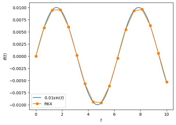

# Again, we can study the convergence of the numerical method

N   = np.array([32, 64, 128, 256, 512, 1024])
E1  = np.array([Err(Euler, n) for n in   N])
E14 = np.array([Err(Euler, n) for n in 4*N])
E2  = np.array([Err(RK2,   n) for n in   N])
E22 = np.array([Err(RK2,   n) for n in 2*N])
E4  = np.array([Err(RK4,   n) for n in   N])

plt.loglog(N, 1/N,    "k--",  label=r"$1/n$")
plt.loglog(N, 1/N**2, "k-.",  label=r"$1/n^2$")
plt.loglog(N, 1/N**4, "k-..", label=r"$1/n^4$")
plt.loglog(N, E1,     "o:",   label=r"Euler")
plt.loglog(N, E14,    "o-",   label=r"Substep Euler")
plt.loglog(N, E2,     "o:",   label=r"RK2")
plt.loglog(N, E22,    "o-",   label=r"Substep RK2")
plt.loglog(N, E4,     "o-",   label=r"RK4")
plt.xlabel(r"$n$")
plt.ylabel(r"$\text{err} = \max|x_\text{numeric} - x|$")
plt.legend()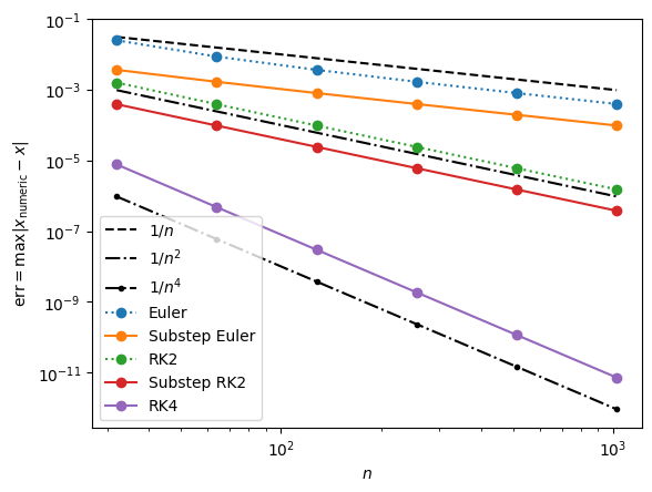

Note that, if one choose $b_1 = 0$ , $b_2 = 1/3$ , $b_3 = 2/3$ , and $b_4 = 1$ , then the solutoin is

\begin{align} (a_1, a_2, a_3, a_4) = \left(\frac{1}{8},\frac{3}{8},\frac{3}{8},\frac{1}{8}\right). \end{align}

(40)

This is Wilhelm Kutta (1901)'s “3/8 method”.

This suggests that Runge-Kutta methods are really a “family”, where many different choices can be used to construct numerical schemes with the same order. The perform of the numerical scheme, nevertheless, depends on the number of oeprations as well as the properties of the ODEs being solved.

# HANDSON: Implement the "3/8 method" and compare it to other ODE
#          integrators that we've implemented.

If we simply update RK4() to use the “3/8 method” coefficients, the resulting algorithm is only 3rd order convergence. This is because RK4() is a special case that, when computing slope $\mathbf{k}_i$ at different time $t_n + b_i \Delta t$ , it depends only on the previous slope $\mathbf{k}_{i-1}$ . In the more general case, $\mathbf{k}_i$ would be a sum of mlutiple previous $\mathbf{k}_j$ for $j < i$ . One would need to go through the full derivation and use the Butcher tableau to implement the algorithm.

Application: Complete Pendulum Problem¶

With a highly accurate ODE integrator like RK4, we are now equipped to solve the complete non-linear gravity pendulum problem. No simplifying assumptions are needed.

def F(x):
    theta, omega = x
    return np.array([omega, -np.sin(theta)])

n  = 1000
dt = 10 / n
X0 = [0, 0.1]
t0 = 0
X4, T4 = RK4(F, X0, t0, dt, n)

Theta4 = X4[:,0]
Omega4 = X4[:,1]

plt.plot(T,  X0[1] * np.sin(T), label=r"$v_0\sin(\theta)$")
plt.plot(T4, Theta4, ':',       label=r"RK4")
plt.xlabel(r"$t$")
plt.ylabel(r"$\theta(t)$")
plt.legend()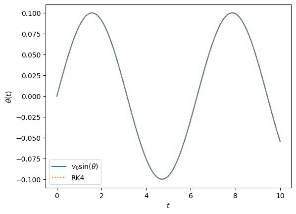

# When the initial velocity is no longer small, the simple harmonic
# oscillator approximation is no longer valid.

n  = 1000
dt = 10 / n
X0 = [0, 1]
t0 = 0
X4, T4 = RK4(F, X0, t0, dt, n)

Theta4 = X4[:,0]
Omega4 = X4[:,1]

plt.plot(T,  X0[1] * np.sin(T), label=r"$v_0\sin(\theta)$")
plt.plot(T4, Theta4, ':',       label=r"RK4")
plt.xlabel(r"$t$")
plt.ylabel(r"$\theta(t)$")
plt.legend()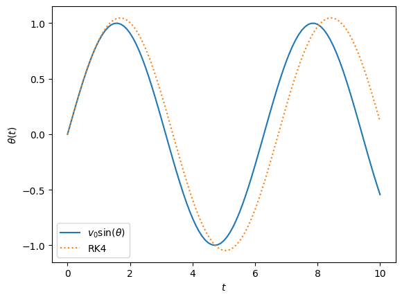

# When the initial velocity is large enough, the solution is not
# periodic.
# What's going on?

n  = 1000
dt = 10 / n
X0 = [0, 2]
t0 = 0
X4, T4 = RK4(F, X0, t0, dt, n)

Theta4 = X4[:,0]
Omega4 = X4[:,1]

plt.plot(T,  X0[1] * np.sin(T), label=r"$v_0\sin(\theta)$")
plt.plot(T4, Theta4, ':',    label=r"RK4")
plt.xlabel(r"$t$")
plt.ylabel(r"$\theta(t)$")
plt.legend()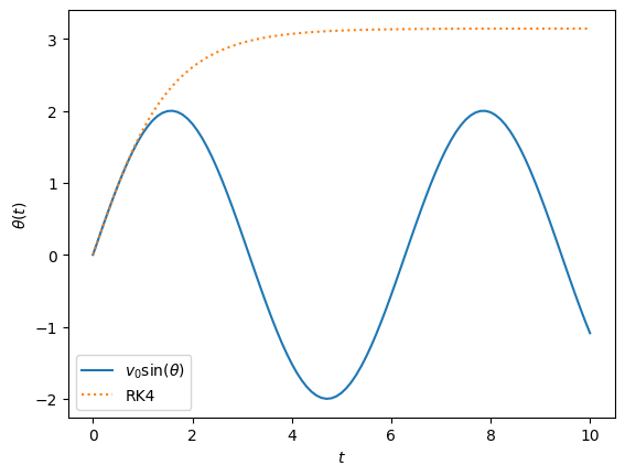

# HANDSON: Try different values of dt and n and observe and initial
#          conditions.

Final Comments¶

Using the insights we developed in numeric integration of functions, we derive multiple ODE integrators. Specifically, we derive the 4th-order Runge-Kutta (RK4) method as a powerful and effective algorithm for solving ordinary differential equations.

The classical RK4 method is not only highly accurate but also robust and relatively simple to implement. When paired with advanced techniques such as adaptive time-stepping and dense output, RK4 becomes even more versatile. This makes RK4 a reliable “workhorse” for ODE integration across many applications.

However, it’s important to remember that there are many other ODE integrators available, each with strengths suited to specific types of equations. For certain problems, especially those involving stiffness or requiring highly efficient, precise computations, other methods may offer better performance. For more information, see resources like Numerical Recipes for additional options and implementation guidance.