Interpolation and Extrapolation

In scientific computing and machine learning, interpolation and extrapolation are essential methods for estimating unknown values from known data.

Interpolation deals with predicting values within the range of available data. This is the foundation of most supervised learning tasks in machine learning, where models predict outputs in the same region where they were trained. Standard interpolation methods include:

Polynomial interpolation is flexible but can suffer from oscillations at the edges of the interval (Runge’s phenomenon).
Rational interpolation can help stabilize the behavior, especially near asymptotes or when functions have strong curvature.
Spline interpolation, particularly cubic splines, provides smooth fits with continuity up to the second derivative. This is especially useful when a smooth curve is required, such as in modeling or visualization.

Extrapolation extends predictions beyond the available data. It is inherently unreliable: without additional information, we cannot know how a function continues beyond the known region. A promising modern approach is physics-informed machine learning (PIML), where physical laws such as ODEs are built into the model. By respecting known constraints, such methods can make extrapolations that remain consistent with physics.

Interpolation and function approximation are related but slightly different. It is useful to distinguish between them:

Interpolation uses existing data to estimate specific missing values.
Function approximation constructs a simplified function that captures the overall behavior of a more complex one. It is often for efficiency or analytic convenience. (See Numerical Recipes, Chapter 5.)

Limitations of Interpolation¶

Even the best interpolation schemes can fail when the function itself is ill-behaved. For example:

\begin{align} f(x) = 3x^2 + \frac{1}{\pi^4}\ln\left[(\pi - x)^2\right] + 1 \end{align}

(1)

This function looks smooth but has a subtle singularity at $x = \pi$ . Interpolating only near the singularity produces misleading results, as we see in these python plots.

import numpy as np

def f(x):
    return 3 * x**2 + np.log((np.pi - x)**2) / np.pi**4 + 1

x1 = np.linspace(3.13, 3.16, 3+1)     # very sparse
x2 = np.linspace(3.13, 3.16, 30+1)    # coarse
x3 = np.linspace(3.13, 3.16, 300+1)   # medium
x4 = np.linspace(3.13, 3.16, 3000+1)  # dense

from matplotlib import pyplot as plt

plt.plot(x4, f(x4),       label='3001 points')
plt.plot(x3, f(x3), '--', label='301 points')
plt.plot(x2, f(x2), 'o:', label='31 points')
plt.plot(x1, f(x1), 'o-', label='4 points')
plt.legend()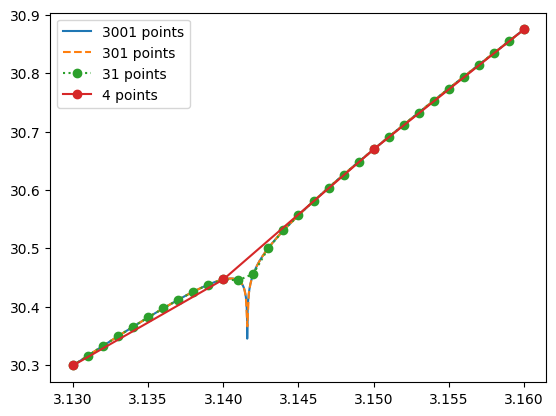

This example shows why interpolation methods should always be paired with error estimates and awareness of the underlying physics or mathematics.

Preliminaries: Searching an Ordered Table¶

Before we can interpolate, we need to know where in the dataset our target value lies. This step is called searching.

If data are sampled on a regular grid, finding neighbors is trivial: just use the array index.
If data are irregularly spaced, we must locate the two points that bracket the target value.
This search step can be just as costly as the interpolation itself, so efficient methods are critical in practice. In fact, in multi-dimension, it may require non-trivial algorithm and advanced data structure.

Numerical Recipes describes two main approaches: bisection and hunting, each suited to different scenarios.

Linear Search¶

As a baseline, let’s consider a simple linear search. It scans through the array until the first value larger than the target is found.

def linear(X, v):
    for i in range(len(X)):  # use a Python loop for clarity
        if X[i] >= v:
            return i - 1

import numpy as np

for _ in range(5):
    X = np.sort(np.random.uniform(0, 100, 10))
    v = np.random.uniform(min(X), max(X))
    i = linear(X, v)
    assert X[i] <= v and v < X[i+1]
    print(f'{X[i]} <= {v} < {X[i+1]}')

31.176133853427235 <= 32.15907636803446 < 36.27845651009813
51.347171865242224 <= 58.461764879790444 < 72.89972903142794
36.59778144585576 <= 68.63864167332986 < 71.93588435564922
57.377788109475944 <= 70.22483207083624 < 74.01039184817246
67.73069335749739 <= 69.00669442703342 < 89.94180991467681

This works, but it requires $\mathcal{O}(N)$ steps. For large datasets, this is inefficient.

Bisection Search¶

The bisection method is much faster. It repeatedly halves the search interval until the target is bracketed. For $N$ data points, it requires only about $\log_2(N)$ steps.

def bisection(X, v):
    l, h = 0, len(X) - 1
    while h - l > 1:
        m = (l + h) // 2
        if v >= X[m]:
            l = m
        else:
            h = m
    return l  # index of the closest value less than the target

for _ in range(5):
    X = np.sort(np.random.uniform(0, 100, 10))
    v = np.random.uniform(min(X), max(X))
    i = bisection(X, v)
    assert X[i] <= v and v < X[i+1]
    print(f'{X[i]} <= {v} < {X[i+1]}')

37.99888228819073 <= 42.499185652948654 < 51.638323796419016
11.82379227474868 <= 17.374282224090496 < 27.174338174003488
11.40445089685429 <= 13.369247320526142 < 13.745558446000594
39.23819803635739 <= 44.556836192533645 < 52.03524182197664
10.471188447832414 <= 12.855689085880513 < 16.369666611374278

This method is robust and efficient for uncorrelated queries, where each target value is unrelated to the previous one.

Hunting Method¶

If target values are requested in sequence and tend to be close to one another, we can do even better. The hunting method exploits this correlation:

Start near the last found index.
Step outward (doubling the step size each time) until the target is bracketed.
Refine the result using bisection in the narrowed interval. This approach is often faster than starting from scratch with bisection every time.

def hunt(X, v, i_last):
    n = len(X)
    assert 0 <= i_last < n - 1

    if v >= X[i_last]:
        l, h, step = i_last, min(n-1, i_last+1), 1
        while h < n - 1 and v > X[h]:
            l, h = h, min(n-1, h + step)
            step *= 2
    else:
        l, h, step = max(0, i_last-1), i_last, 1
        while l > 0 and v < X[l]:
            l, h = max(0, l - step), l
            step *= 2

    return bisection(X[l:h+1], v) + l

for _ in range(5):
    X = np.sort(np.random.uniform(0, 100, 10))
    v = np.random.uniform(min(X), max(X))
    i = bisection(X, v)
    assert X[i] <= v and v < X[i+1]
    print(f'{X[i]} <= {v} < {X[i+1]}')

67.81439792226539 <= 78.86293657654261 < 92.55144568182011
26.876524441692307 <= 37.5502953237929 < 38.54773220555812
52.69595734468182 <= 79.1278418612532 < 90.1322012882293
28.806570771514327 <= 36.80827889978012 < 42.07916185528746
41.389681727978775 <= 44.943774525675664 < 48.27748179305923

Linear Interpolation with Searching¶

With a search routine in place, interpolation becomes straightforward. Below is a simple interpolator that supports hunt, bisection, or linear searching.

class Interpolator:
    
    def __init__(self, X, Y):
        assert len(X) == len(Y)
        self.X, self.Y = X, Y
        self.i_last = len(X) // 2

    def __call__(self, v, method='hunt'):
        if method == 'hunt':
            i = hunt(self.X, v, self.i_last)
        elif method == 'bisection':
            i = bisection(self.X, v)
        else:
            i = linear(self.X, v)

        self.i_last = i  # store last index for hunting

        x0, x1 = self.X[i], self.X[i+1]
        y0, y1 = self.Y[i], self.Y[i+1]
        m      = (y1 - y0) / (x1 - x0)
        return y0 + m * (v - x0)

import matplotlib.pyplot as plt

def f(x):
    return np.exp(-0.5 * x**2)

Xs = np.sort(np.random.uniform(-5, 5, 20))
Ys = f(Xs)

fi = Interpolator(Xs, Ys)

Xi = np.linspace(min(Xs), max(Xs), 100)
Yi = np.array([fi(x) for x in Xi])

plt.plot(Xs, Ys, 'o-', label='Sampled data')
plt.plot(Xi, Yi, '.',  label='Interpolation')
plt.legend()
plt.show()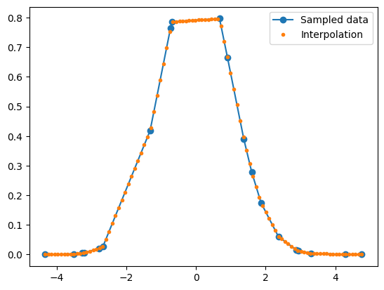

Finally, let’s test our claim: hunting should be faster than bisection when queries are sequential and correlated.

from timeit import timeit

Xs = np.sort(np.random.uniform(-5, 5, 1000))
Ys = f(Xs)
fi = Interpolator(Xs, Ys)
Xi = np.linspace(min(Xs), max(Xs), 10_000)

def job(method):
    Yi = [fi(x, method) for x in Xi]

dt_linear    = timeit("job('linear')",    globals=globals(), number=1)
dt_bisection = timeit("job('bisection')", globals=globals(), number=1)
dt_hunt      = timeit("job('hunt')",      globals=globals(), number=1)

print('Linear   :', dt_linear)
print('Bisection:', dt_bisection)
print('Hunt     :', dt_hunt)

Linear   : 0.6211810980021255
Bisection: 0.03016846200625878
Hunt     : 0.01707720999547746

# HANDSON: change the number of sampled points and interpolation
#          points and measure the performance of all three methods.
#          What are the performance characteristics when
#          N_sample >> N_interpolation and
#          N_sample << N_interpolation?

Main Take Away

It may seem surprising that interpolation, which sounds like purely numerical, actually spends much of its effort on searching. The interpolation formula itself is simple, but locating the right interval in the data dominates the work.

This may be less surprising if we start asking ourselves what are computers good at? Certainly at arithmetic, but equally at bookkeeping (and communication now when we have internet). In fact, much of computer science is devoted to studying how to organize and retrieve data efficiently. This is what “data structures and algorithms” are about. Searching in interpolation is a great example of this. Efficient bookkeeping can matter as much as the numerical formula.

Our codes here were one-dimensional and simple. But in practice, many scientific applications require multidimensional interpolation. In higher dimensions, the search problem quickly becomes far more complicated. Efficient methods often rely on tree structures (e.g., kd-trees or octrees) to organize points and make search practical. This is the same kind of complexity that appears in $n$ -body simulations and particle-mesh algorithms, where bookkeeping and efficient search dominate performance.

Thus, linear interpolation serves as a small but important lesson: computational science (i.e., numerical analysis) and computer science are deeply connected. To do science at scale, one must care not only about the equations, but also about how data are organized and searched.

Polynomial Interpolation and Extrapolation¶

Given $M$ data points $(x_0, y_0), (x_1, y_1), \dots, (x_{M-1}, y_{M_1})$ , there exists a unique polynomial of degree $M-1$ that passes through all of them exactly.

Lagrange’s Formula¶

The classical formula due to Lagrange writes this polynomial as

\begin{align} P_{M-1}(x) &= \frac{(x-x_1)(x-x_2)\dots(x-x_{M-1})}{(x_0-x_1)(x_0-x_2)\dots(x_0-x_{M-1})} y_0 \\ &+ \frac{(x-x_0)(x-x_2)\dots(x-x_{M-1})}{(x_1-x_0)(x_1-x_2)\dots(x_1-x_{M-1})} y_1 + \dots \\ &+ \frac{(x-x_0)(x-x_2)\dots(x-x_{M-2})}{(x_{M-1}-x_0)(x_{M-1}-x_1)\dots(x_{M-1}-x_{M-2})} y_{M-1}. \end{align}

(2)

Using summation and product notation, we can write this more compactly as

\begin{align} P_{M-1}(x) = \sum_{m=0}^{M-1} \frac{\prod_{n=0,n\ne m}^{M-1}(x-x_n)}{\prod_{n=0,n\ne m}^{M-1}(x_m-x_n)} y_m. \end{align}

(3)

It is straightforward to check that substituting $x = x_{m'}$ gives

\begin{align} P_{M-1}(x_{m'}) = \sum_{m=0}^{M-1} \delta_{mm'} y_m \end{align}

(4)

so the polynomial indeed passes through all the data points.

Neville’s Algorithm¶

While Lagrange’s formula is mathematically elegant, it is not the most practical for computation:

It does not directly provide an error estimate.
It requires recomputation for each new interpolation point. A better approach is Neville’s Algorithm, which recursively builds the interpolating polynomial and naturally provides error estimates. This makes it especially useful for small to moderate datasets.

Step 1: Zero-Degree Polynomials¶

A polynomial of degree 0 is just a constant. For each data point $(x_m, y_m)$ , define

\begin{align} P_m(x) = y_m \end{align}

(5)

These form the base case for the recursion.

Xs = np.sort(np.random.uniform(-5, 5, 100))
Ys = f(Xs)

plt.scatter(Xs, Ys, marker='_', color='C0', label=r'$P_m$: polynomials with 0 degree')
plt.xlim(-0.5, 0.5)
plt.ylim( 0.9, 1.05)
plt.legend()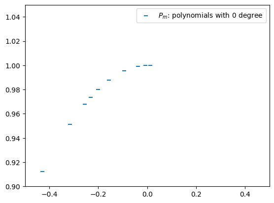

Step 2: First-Degree Polynomials¶

We now interpolate between two neighboring points $(x_{m'}, y_{m'})$ and $(x_{m'+1}, y_{m'+1})$ . This gives a linear polynomial, denoted $P_{m',m'+1}(x)$ :

\begin{align} \frac{P_{m',m'+1} - P_{m'}}{x - x_{m'}} &= \frac{P_{m'+1} - P_{m'}}{x_{m'+1} - x_{m'}} \\ P_{m',m'+1} - P_{m'} &= \frac{x - x_{m'}}{x_{m'+1} - x_{m'}}(P_{m'+1} - P_{m'}) \\ P_{m',m'+1} &= P_{m'} + \frac{x - x_{m'}}{x_{m'+1} - x_{m'}}(P_{m'+1} - P_{m'}) \\ P_{m',m'+1} &= \frac{x_{m'+1} - x_{m'}}{x_{m'+1} - x_{m'}}P_{m'} + \frac{x - x_{m'}}{x_{m'+1} - x_{m'}}(P_{m'+1} - P_{m'}) \\ P_{m',m'+1} &= \left(\frac{x_{m'+1} - x_{m'}}{x_{m'+1} - x_{m'}} - \frac{x - x_{m'}}{x_{m'+1} - x_{m'}}\right)P_{m'} + \frac{x - x_{m'}}{x_{m'+1} - x_{m'}}P_{m'+1} \\ P_{m',m'+1} &= \frac{x_{m'+1} - x}{x_{m'+1} - x_{m'}}P_{m'} + \frac{x - x_{m'}}{x_{m'+1} - x_{m'}}P_{m'+1} \\ P_{m',m'+1} &= \frac{(x - x_{m'+1})P_{m'} + (x_{m'} - x)P_{m'+1} }{x_{m'} - x_{m'+1}} \end{align}

(6)

This is simply the two-point form of a line.

Pmm1s = []
for m in range(len(Xs)-1):
    Pmm1s.append(lambda x: ((x - Xs[m+1]) * Ys[m] + (Xs[m] - x) * Ys[m+1]) / (Xs[m] - Xs[m+1]))

plt.scatter(Xs, Ys, marker='_', color='C0', label=r'$P_m$: polynomials with 0 degree')

label = r'$P_{m,m+1}$: polynomials with 1 degree'
for m, Pmm1 in enumerate(Pmm1s):
    xs = np.linspace(Xs[m], Xs[m+1], 100)
    ys = Pmm1(xs)
    plt.plot(xs, ys, color='C1', label=label)
    label = None

plt.xlim(-0.5, 0.5)
plt.ylim( 0.9, 1.05)
plt.legend()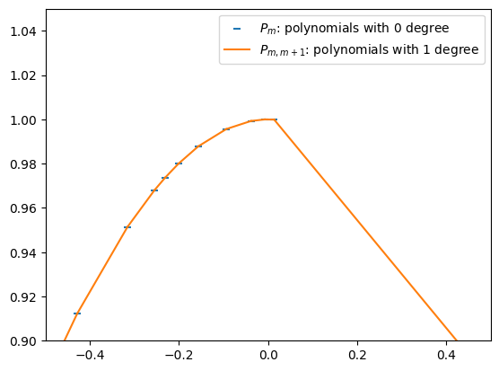

Step 3: Second-Degree Polynomials¶

By interpolating two neighboring first-degree polynomials, we obtain a second-degree polynomial:

\begin{align} P_{m'',m''+1,m''+2} &= \frac{(x - x_{m''+2})P_{m'',m''+1} + (x_{m''} - x)P_{m''+1,m''+2} }{x_{m'} - x_{m'+2}}. \end{align}

(7)

Pmm1m2s = []
for m in range(len(Xs)-2):
    Pmm1  = lambda x: ((x - Xs[m+1]) * Ys[m  ] + (Xs[m  ] - x) * Ys[m+1]) / (Xs[m  ] - Xs[m+1])
    Pm1m2 = lambda x: ((x - Xs[m+2]) * Ys[m+1] + (Xs[m+1] - x) * Ys[m+2]) / (Xs[m+1] - Xs[m+2])
    Pmm1m2s.append(
        lambda x: ((x - Xs[m+2]) * Pmm1(x) + (Xs[m] - x) * Pm1m2(x)) / (Xs[m] - Xs[m+2])
    )

plt.scatter(Xs, Ys, marker='o', color='C0', label=r'$P_m$: polynomials with 0 degree')

label = r'$P_{m,m+1}$: polynomials with 1 degree'
for m, Pmm1 in enumerate(Pmm1s[:-1]):
    xs = np.linspace(Xs[m], Xs[m+1], 100)
    ys = Pmm1(xs)
    plt.plot(xs, ys, color='C1', label=label)
    label = None

label = r'$P_{m,m+1,m+2}$: polynomials with 2 degree'
for m, Pmm1m2 in enumerate(Pmm1m2s):
    xs = np.linspace(Xs[m], Xs[m+1], 100)
    ys = Pmm1m2(xs)
    plt.plot(xs, ys, ':', color='C2', label=label)
    label = None

plt.xlim(-0.5, 0.5)
plt.ylim( 0.9, 1.05)
plt.legend()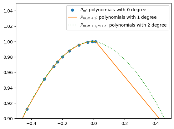

Step 4: Recursive Formula¶

By continuing this process, we arrive at the general recursive formula for Neville’s algorithm (Numerical Recipes Eq. 3.2.3):

\begin{align} P_{m,m+1,\dots,m+n} &= \frac{(x - x_{m+n})P_{m,m+1,\dots,m+n-1} + (x_{m} - x)P_{m+1,m+2,\dots,m+n} }{x_{m} - x_{m+n}}. \end{align}

(8)

This provides a systematic way to build higher-order interpolating polynomials.

Step 5: Avoiding Catastrophic Cancellation¶

Direct implementation of the above formulations may suffer from catastrophic cancellation, especially when points are close together. Numerical Recipes reformulates the recursion in terms of small corrections $C_{n,m}$ and $D_{n,m}$ :

\begin{align} C_{n,m} &\equiv P_{m,m+1,\dots,m+n} - P_{m,m+1,\dots,m+n-1} \\ D_{n,m} &\equiv P_{m,m+1,\dots,m+n} - P_{m+1,m+2,\dots,m+n} \end{align}

(9)

These track the incremental updates that improve accuracy.

Neville’s algorithm can now be rewritten as

\begin{align} D_{n+1,m} &= \frac{x_{m+n+1}-x}{x_m - x_{m+n+1}}(C_{n,m+1} - D_{n,m}) \\ C_{n+1,m} &= \frac{x_{n}-x}{x_m - x_{m+n+1}}(C_{n,m+1} - D_{n,m}) \end{align}

(10)

From this expression, it is now clear that the $C$ ’s and $D$ ’s are the corrections that make the interpolation one order higher.

Step 6. Implementation¶

The final polynomial $P_{0,1,\dots,M-1}$ is equal to the sum of any $y_i$ plus a set of $C$ ’s and/or $D$ ’s that form a path through the family tree of $P_{m,m+1,\dots,m+n}$ .

class PolynomialInterpolator:
    
    def __init__(self, Xs, Ys, n=None):
        if n is None:
            n = len(Xs)

        assert len(Xs) == len(Ys)
        assert len(Xs) >= n

        self.Xs, self.Ys, self.n = Xs, Ys, n

    def __call__(self, target, search_method='hunt'):

        C = np.copy(self.Ys)
        D = np.copy(self.Ys)

        i = np.argmin(abs(self.Xs - target))
        y = self.Ys[i]
        i-= 1

        for n in range(1,self.n):
            ho  = self.Xs[:-n] - target
            hp  = self.Xs[+n:] - target
            w   = C[1:self.n-n+1] - D[:-n]
            den = ho - hp
            if any(den == 0):
                raise Exception("two input Xs are (to within roundoﬀ) identical.")
            else:
                f = w / den
            D[:-n] = hp * f
            C[:-n] = ho * f

            if 2*(i+1) < (self.n-n):
                self.dy = C[i+1]
            else:
                self.dy = D[i]
                i -= 1

            y += self.dy

        return y

Xs = np.linspace(-1,1,21)
Ys = f(Xs)

P  = PolynomialInterpolator(Xs, Ys)

Xi = np.linspace(min(Xs),max(Xs),201)
Yi = []
Ei = []
for x in Xi:
    Yi.append(P(x))
    Ei.append(P.dy)
Yi = np.array(Yi)
Ei = np.array(Ei)

fig, axes = plt.subplots(2,1,figsize=(8,6))
axes[0].scatter(Xs, Ys)
axes[0].plot(Xi, Yi, '-', color='r')
axes[1].semilogy(Xi, abs(Ei))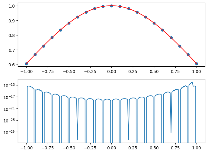

# HANDSON: Change the sampling points to, e.g.,
#
#              Xs = np.linspace(-5,5,21)
#              Xs = -5 * np.cos(np.linspace(0, np.pi, 21))
#
#          How does the error converge if we increase (or decrease)
#          the number of sampling points?
#          What will happen if we increase the size of the domain?
#          (This is called Runge phenomenon.)
#          What will happen if we try to extrapolate?

# HANDSON: Our interpolator can take different order of
#          approximations.
#          Create convergence plots and study the error as function of
#          the order.
#          What happen when we have different domain size?
#          What happen when we have different sampling points?

More Interpolation Algorithms¶

For further study, here are several powerful alternatives and extensions to polynomial interpolation:

Cubic Splines: Ensure smoothness across intervals by matching derivatives at knots, avoiding the oscillations of high-degree polynomials.
Rational Function Interpolation: Use ratios of polynomials to capture asymptotic behavior and improve stability.
Direct Polynomial Coefficients: Compute coefficients efficiently (e.g., via Newton’s form) when polynomials are truly required.
Multidimensional Interpolation: Extend interpolation to higher dimensions, important for applications such as spatial data analysis and numerical simulations.
Laplace Interpolation: A specialized technique for harmonic functions, using properties of Laplace’s equation.

Interpolation is not one-size-fits-all. Polynomial methods are elegant and instructive, but understanding their strengths and weaknesses is important. By combining them with more advanced techniques, we can handle a much wider range of problems in scientific computing.

Instead of re-deriving or implementing all of these algorithms from scratch, we will try out a few of them using built-in functions from numpy and scipy. This will give us hands-on experience with practical tools while reinforcing the ideas we have discussed.

Cubic Splines¶

The classical choice for smooth interpolation is the cubic spline. It guarantees continuity of the function, its first derivative, and its second derivative across intervals.

from scipy.interpolate import CubicSpline, PchipInterpolator

Xs = np.sort(np.random.uniform(-3, 3, 100))
Ys = f(Xs)

CS    = CubicSpline(Xs, Ys)        # classical cubic spline
Pchip = PchipInterpolator(Xs, Ys)  # monotone, shape-preserving

Xi = np.linspace(-3, 3, 1000)

plt.plot(Xi, f(Xi),     'k',  label='true f(x)')
plt.plot(Xs, Ys,        'o',  label='data')
plt.plot(Xi, CS(Xi),    '--', label='CubicSpline')
plt.plot(Xi, Pchip(Xi), ':',  label='PCHIP')
plt.legend()

plt.xlim(-0.5, 0.5)
plt.ylim( 0.9, 1.05)

(0.9, 1.05)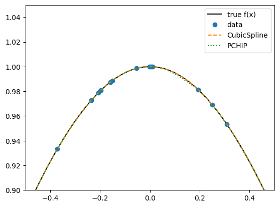

# HANDSON: add some noise to the data and compare `CubicSpline`
#          vs. `PchipInterpolator`.
#          Which one is more robust against oscillations?

Multidimensional Interpolation¶

Interpolation often appears in 2D or 3D. SciPy provides two useful tools:

griddata: works with scattered data.
RegularGridInterpolator: efficient for regular grids.

from scipy.interpolate import griddata

Xs = np.random.uniform(-3, 3, 100)
Ys = np.random.uniform(-3, 3, 100)
Zs = f(np.sqrt(Xs * Xs + Ys * Ys))

# Interpolate on a grid
Xg, Yg = np.meshgrid(
    np.linspace(-3, 3, 301),
    np.linspace(-3, 3, 301),
    indexing='xy')
Zg = griddata((Xs, Ys), Zs, (Xg, Yg), method='cubic')

plt.imshow(Zg, extent=[-3,3,-3,3], origin='lower')
plt.colorbar(label='Interpolated value')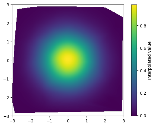

# HANDSON: 
#
# 1. Why is the outer shape of the plot irregular?
#
# 2. Adjust the number of sampling points and interpolation points.
#    How does the resulting plots look like?
#
# 3. Try methods 'linear', 'nearest', and 'cubic'.
#    Compare smoothness vs. accuracy.

# HANDSON: try to use `RegularGridInterpolator` to interpolate on a
#          regular grid.