Data Representation and Round-Off Errors

Representing Integers¶

Efficient number representation, as illustrated in the riddle, enables us to solve seemingly impossible problems. The evolution of numeral systems reflects humanity’s progress toward clarity and efficiency in expressing information.

Unary System: The simplest system, where each number is represented by identical marks. For example, 5 is written as “|||||”. While easy to understand and requiring no skill for addition, unary becomes impractical for large values: representing 888 requires 888 marks.
Roman Numerals: An improvement over unary, Roman numerals use symbols such as I (1), V (5), X (10), L (50), C (100), D (500), and M (1000) to group large values. However, representing numbers like 888 (DCCCLXXXVIII) still requires 12 symbols, which is somewhat cumbersome.
Arabic Numerals: We may take it for granted and not appreciate it, but Arabic numeral system is a revolutionary advancement. It uses positional notation to represent numbers compactly and efficiently. For instance, 888 requires only three digits.

Positional Notation Systems¶

The Arabic numeral system is an example of a positional notation system, where the value of a digit is determined by both the digit itself and its position within the number. This contrasts with systems like unary numbers or Roman numerals, where the position of a symbol does not affect its value. In positional notation, each digit’s place corresponds to a specific power of the system’s base.

In a positional system, representing a number involves the following steps:

Decide on the base (or radix) $b$ .
Define the notation for the digits.
Write the number as:
$\begin{align} \pm (\dots d_3 d_2 d_1 d_0 . d_{-1} d_{-2} d_{-3} \dots), \end{align}$
(1)
which represents:
$\begin{align} \pm (\dots + d_3 b^3 + d_2 b^2 + d_1 b^1 + d_0 b^0 + d_{-1} b^{-1} + d_{-2} b^{-2} + d_{-3} b^{-3} + \dots). \end{align}$
(2)

To convert a number from base $b$ to decimal, we apply this definition directly. For example:

\begin{align} (256.4)_8 = 2\times8^2 + 5\times8^1 + 6\times8^0 + 4\times8^{-1} = (174.5)_{10}. \end{align}

(3)

The most popular bases used in computer are:

Binary Numbers¶

Base: $b = 2$
Digits: 0, 1

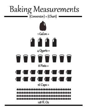
Binary system was invented by merchants in medieval England

The binary system has been used in various forms long before the age of computers. Invented by merchants in medieval England, the units of liquid measure were based on the binary system. For example:

1 gallon = 2 pottles;
1 pottle = 2 quarts;
1 quart = 2 pints;
1 pint = 2 cups; etc.

Similarly, the binary system is used in music to define note durations, i.e., whole note, half note, quarter note, eighth note, sixteenth note, etc. These everyday examples show the fundamental nature of the binary system underpining modern computing.

There are 10 types of people in the world...

In the binary system, only two digits are used: 0 and 1. The position of each digit in a binary number corresponds to a power of 2, just as the position of a digit in the decimal system corresponds to a power of 10. For example, the binary number 1011₂ represents: $1 \times 2^3 + 0 \times 2^2 + 1 \times 2^1 + 1 \times 2^0$ . This gives the decimal value: $1 \times 8 + 0 \times 4 + 1 \times 2 + 1 \times 1 = 11$ .

In Python, you can use the bin() function to convert an integer to its binary string representation, and the int() function to convert a binary string back to an integer. This is particularly useful when working with binary numbers in computations.

# Convert an integer to a binary string
number = 10
binary = bin(number)

print(f"Binary representation of {number}: {binary}")

Binary representation of 10: 0b1010

# Convert a binary string back to an integer
binary = "0b1010" # the leading "0b" is optional
number = int(binary, 2)

print(f"Integer value of {binary}: {number}")

Integer value of 0b1010: 10

Note that the above examples use formatted string literals, commonly known as “f-strings.” F-strings provide a concise and readable way to embed expressions inside string literals by prefixing the string with an f or F character.

Python supports representing binary numbers directly using the 0b prefix for literals. This allows you to define binary numbers without converting from a string format.

binary = 0b1010  # 10 in decimal

print(f"Binary number: {binary}")

Binary number: 10

The Hexadecimal System¶

Base: $b = 16$
Digits: 0, 1, 2, 3, 4, 5, 6, 7, 8, 9, A, B, C, D, E, F

The hexadecimal system allows for writing a binary number in a very compact notation. It allows one to directly ready the binary content of a file, e.g.,

% hexdump -C /bin/sh | head
00000000  ca fe ba be 00 00 00 02  01 00 00 07 00 00 00 03  |................|
00000010  00 00 40 00 00 00 6a b0  00 00 00 0e 01 00 00 0c  |..@...j.........|
00000020  80 00 00 02 00 00 c0 00  00 00 cb 70 00 00 00 0e  |...........p....|
00000030  00 00 00 00 00 00 00 00  00 00 00 00 00 00 00 00  |................|
*
00004000  cf fa ed fe 07 00 00 01  03 00 00 00 02 00 00 00  |................|
00004010  11 00 00 00 c0 04 00 00  85 00 20 00 00 00 00 00  |.......... .....|
00004020  19 00 00 00 48 00 00 00  5f 5f 50 41 47 45 5a 45  |....H...__PAGEZE|
00004030  52 4f 00 00 00 00 00 00  00 00 00 00 00 00 00 00  |RO..............|
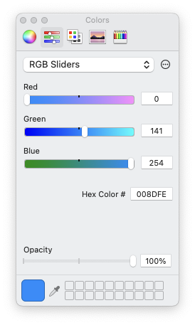
00004040  00 00 00 00 01 00 00 00  00 00 00 00 00 00 00 00  |................|

or directly select a color

Python also supports working with hexadecimal numbers, which are represented using the 0x prefix. Below are examples demonstrating how to handle hexadecimal numbers in Python.

number = 255
hexrep = hex(number)

print(f"Hexadecimal representation of {number}: {hexrep}")

Hexadecimal representation of 255: 0xff

hexrep = "0xff"
number = int(hexrep, 16)

print(f"Integer value of {hexrep}: {number}")

Integer value of 0xff: 255

hexrep = 0xff  # 10 in decimal

print(f"Hexadecimal number: {hexrep}")

Hexadecimal number: 255

Quantum Computing: A New Type of Number Representation

Quantum computing takes number representation to a whole new level. In quantum mechanics, data is represented using quantum bits, or qubits. Unlike classical bits, a single qubit can exist in a superposition of two states, $|0\rangle$ and $|1\rangle$ , simultaneously. This means that (ignoring normalization for now) one qubit can represent two numbers $C_0$ and $C_1$ as in $C_0 |0\rangle + C_1 |1\rangle$ .

With two qubits, the system can represent four possible states: $|00\rangle$ , $|01\rangle$ , $|10\rangle$ , and $|11\rangle$ , again, in superposition. The number of possible states grows exponentially as more qubits are added:

Three qubits can represent eight states: $|000\rangle$ , $|001\rangle$ , $|010\rangle$ , ..., $|111\rangle$ .
Four qubits represent 16 states, and so on.

In general, $n$ qubits can represent $2^n$ states at once. This exponential scaling is what gives quantum computers their enormous potential to perform certain types of calculations far more efficiently than classical computers.

For example, IBM’s 53-qubit quantum computer can represent 2⁵³ states simultaneously. In terms of classical information, this is equivalent to storing approximately 1 petabyte (PB) of data, which is comparable to the amount of memory available in some of the world’s largest supercomputers today.

Superposition Hypothesis in Large Language Models

The Superposition Hypothesis in large language models (LLMs) proposes that individual neurons or parameters can encode multiple overlapping features, depending on context. This is analogous to quantum superposition, where qubits represent multiple states simultaneously.

For example, a single neuron in an LLM might activate for both “dog” and “pet,” enabling efficient reuse of parameters.

This ability is further supported by high-dimensional embeddings, where concepts are represented as nearly orthogonal vectors. This allows the LLM to store and distinguish vast amounts of information with minimal interference. The Johnson-Lindenstrauss Lemma explains how high-dimensional spaces accommodate such efficient representations.

While the Superposition Hypothesis provides a promising explanation for the efficiency of LLMs, it remains an area of active research to fully understand the mechanisms underlying their success.

Hardware Implementations¶

The decimal system has been established, somewhat foolishly to be sure, according to man’s custom, not from a natural necessity as most people think.
- Blaise Pascal (1623--1662)

Binary operators are the foundation of computation in digital hardware.

Basic Binary Operators¶

AND Operator (&)

| A | B | A & B |
|---|---|-------|
| 0 | 0 |   0   |
| 0 | 1 |   0   |
| 1 | 0 |   0   |
| 1 | 1 |   1   |

OR Operator (|)

| A | B | A | B |
|---|---|-------|
| 0 | 0 |   0   |
| 0 | 1 |   1   |
| 1 | 0 |   1   |
| 1 | 1 |   1   |

XOR Operator (^)

| A | B | A ^ B |
|---|---|-------|
| 0 | 0 |   0   |
| 0 | 1 |   1   |
| 1 | 0 |   1   |
| 1 | 1 |   0   |

NOT Operator (~)

| A | ~A |
|---|----|
| 0 |  1 |
| 1 |  0 |

NAND and NOR Operators
- NAND (NOT AND): Outputs 0 only when both inputs are 1.
- NOR (NOT OR): Outputs 1 only when both inputs are 0.

CMOS Implementation¶

Logic gates are built using CMOS (Complementary Metal-Oxide-Semiconductor) technology, which utilizes:

PMOS Transistors: Conduct when the input is low (logic 0).
NMOS Transistors: Conduct when the input is high (logic 1).

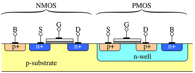
Cross section of two transistors in a CMOS gate, in an N-well CMOS process.

In the above figure, the terminals of the transistors are labeled as follows:

Source (S): The terminal where carriers (electrons or holes) enter the transistor. For NMOS transistors, the source is typically connected to a lower potential (e.g., ground), while for PMOS transistors, it is connected to a higher potential (e.g., Vdd).
Gate (G): The terminal that controls the flow of carriers between the source and drain. Applying a voltage to the gate creates an electric field that either allows or prevents current flow, effectively acting as a switch.
Drain (D): The terminal through which carriers exit the transistor. For NMOS transistors, the drain is usually connected to a higher potential, while for PMOS transistors, it is connected to a lower potential.
Body (B): Also known as the bulk or substrate, this terminal is typically connected to a fixed reference potential. For NMOS transistors, the body is often connected to ground, and for PMOS transistors, it is connected to Vdd. The body helps control leakage currents and influences the transistor’s threshold voltage.

By manipulating the voltage at the gate terminal, transistors act as switches. They then enable or disable the flow of current between the source and drain. This non-linear switching behavior supports the operation of all logic gates and digital circuits.

Here are some CMOS Gate Examples

NOT Gate:
- PMOS: Connects the output to Vdd (high) when the input is low.
- NMOS: Connects the output to ground (low) when the input is high.
NAND Gate:
- PMOS: Two transistors in parallel connect to Vdd if either input is low.
- NMOS: Two transistors in series connect to ground only if both inputs are high.
NOR Gate:
- PMOS: Two transistors in series connect to Vdd only if both inputs are low.
- NMOS: Two transistors in parallel connect to ground if either input is high.

Universal Gates¶

NAND and NOR gates are also called universal gates because any other logic gate can be constructed using just these gates. Universal gates are fundamental in hardware design, as they simplify manufacturing by reducing the variety of components needed.

In practice, the NAND gate is widely used in the industry due to several advantages:

Less delay
Smaller silicon area
Uniform transistor sizes

An NAND gate’s truth table looks like this:

| A | B | NAND(A, B) |
|---|---|------------|
| 0 | 0 | 1          |
| 0 | 1 | 1          |
| 1 | 0 | 1          |
| 1 | 1 | 0          |

Here is a simple Python function for the NAND gate:

def NAND(a, b):
    return 1 - (a & b)  # NOT (a AND b)

We can now construct basic gates using only NAND:

# A NOT gate can be built by connecting both inputs of a NAND gate to the same value.

def NOT(a):
    return NAND(a, a)

# Test
print(NOT(0)) # Output: 1
print(NOT(1)) # Output: 0

1
0

# An AND gate can be built by negating the output of a NAND gate.

def AND(a, b):
    return NOT(NAND(a, b))

# Test
print(AND(0, 0))  # Output: 0
print(AND(0, 1))  # Output: 0
print(AND(1, 0))  # Output: 0
print(AND(1, 1))  # Output: 1

# HANDSON: implement an OR gate using only NAND.
#
# HINT: Using De Morgan's law: A | B = ~(~A & ~B).

def OR(a, b):
    return NAND(NOT(a), NOT(b))

# Test
print(OR(0, 0))  # Output: 0
print(OR(0, 1))  # Output: 1
print(OR(1, 0))  # Output: 1
print(OR(1, 1))  # Output: 1

# HANDSON: implement an XOR gate using only NAND.

def XOR(a, b):
    c = NAND(a, b)
    return NAND(NAND(a, c), NAND(b, c))

# Test
print(XOR(0, 0))  # Output: 0
print(XOR(0, 1))  # Output: 1
print(XOR(1, 0))  # Output: 1
print(XOR(1, 1))  # Output: 0

Addition in the Binary System¶

In the binary system, addition follows similar rules to decimal addition, but with only two digits: 0 and 1. The key rules are:

0 + 0 = 0
0 + 1 = 1
1 + 0 = 1
1 + 1 = 0, 1 carryover

We start from the rightmost bit, adding the bits with carry when needed:

    C = 111
    A = 0101 (  A = 5)
    B = 0011 (  B = 3)
-------------
A + B = 1000 (A+B = 8)

Half Adder: Building Blocks for Addition¶

A half adder is a fundamental circuit used to add two single-bit binary numbers. It produces two outputs:

Sum: The result of the XOR operation between the two inputs.
Carry: The result of the AND operation between the two inputs, representing an overflow to the next bit.

However, the half adder is limited because it does not account for a carry input from a previous addition. This is why it is called a “half” adder---it handles only the addition of two bits without any carry forwarding.

The logic for a half adder can be represented as:

A + B = S , C
-------------
0 + 0 = 0 , 0
0 + 1 = 1 , 0
1 + 0 = 1 , 0
1 + 1 = 0 , 1

This simplicity makes the half adder a foundational component for building more complex adders, like the full adder.

def half_adder(A, B):
    S = XOR(A, B)  # Sum using XOR
    C = AND(A, B)  # Carry using AND
    return S, C

# Test
print(half_adder(0, 0))
print(half_adder(0, 1))
print(half_adder(1, 0))
print(half_adder(1, 1))

(0, 0)
(1, 0)
(1, 0)
(0, 1)

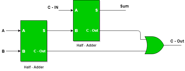
Building a Full Adder Using NAND¶

A full adder extends the half adder by adding a carry input. It is capable of handling three inputs:

A: First bit
B: Second bit
Cin: Carry from the previous bit addition

It produces two outputs:

S: Result of adding A, B, and Cin.
Cout: Overflow to the next higher bit.

It can be implemented using two half adder and an OR gate:

def full_adder(A, B, Cin):
    s, c = half_adder(A,   B)
    S, C = half_adder(Cin, s)
    Cout = OR(c, C)
    return S, Cout

# Test
print(full_adder(0, 0, 0))  # Output: (0, 0)
print(full_adder(1, 0, 0))  # Output: (1, 0)
print(full_adder(1, 1, 0))  # Output: (0, 1)
print(full_adder(1, 1, 1))  # Output: (1, 1)

(0, 0)
(1, 0)
(0, 1)
(1, 1)

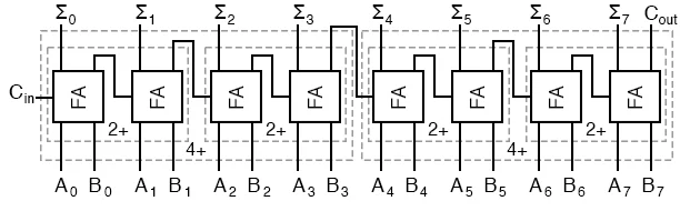
Multi-Bit Adder¶

A multi-bit adder combines multiple full adders to add two binary numbers of arbitrary length. Each full adder handles one bit, with the carry output of one adder serving as the carry input to the next.

For example, to add two 4-bit binary numbers A3 A2 A1 A0 and B3 B2 B1 B0:

Set the initial carry to 0
Use full adders for all bits. Then, we can combine multiple full adders to make multi-bit adders.

def multibit_adder(A, B, carrybit=False):
    assert(len(A) == len(B))
    
    n = len(A)
    c = 0
    S = []
    for i in range(n):
        s, c = full_adder(A[i], B[i], c)
        S.append(s)
    if carrybit:
        S.append(c)  # add the extra carry bit
    return S

# Test
A = [1, 1, 0, 1]  # 1 + 2 + 8 = 11 in binary
B = [1, 0, 0, 1]  # 1 + 8 = 9 in binary
print(multibit_adder(A, B, carrybit=True))  # Output: [0, 0, 1, 0, 1] = 4 + 16 = 20 in binary

[0, 0, 1, 0, 1]

Number of Bits in an Integer¶

The number of bits used to store an integer determines the range of values it can represent.

For unsigned integers, the range is $[0, 2^b - 1]$ , where $b$ is the number of bits.
For signed integers, one bit is used for the sign, leaving $n-1$ bits for the value. The range for signed integers is usually $[-2^{n-1}, 2^{n-1} - 1]$ (see below).

For example:

An 8-bit unsigned integer represents values from 0 to 255.
An 8-bit signed integer represents values from -128 to 127.

In modern programming languages, integers may be implemented as fixed-width (e.g., 8, 16, 32, 64 bits) or variable-width types.

Overflow and Underflow Error¶

The multibit_adder() example above clearly shows that adding two $b$ -bit integer may result a $(b+1)$ -bit integer.

In computing, overflow error occurs when an integer calculation exceeds the maximum value that can be represented within the allocated number of bits. For example, in a 32-bit unsigned integer, the maximum value is $2^{32} - 1$ (= 4,294,967,295). Adding 1 to this value causes the result to “wrap around” to the minimum value 0. Similarly, underflow occurs when subtracting below the minimum value.

To mitigate these errors, some programming languages and compilers provide tools to detect overflow or implement arbitrary-precision integers, which grow dynamically to store larger values. Specifically, Python’s int is unbounded and dynamically adjusts to the size of the number.

Representation of Negative Numbers¶

The most common method in modern computer to represent negative integers is two’s complement, where:

Positive numbers are represented as usual in binary.
To represent a negative number:
- Write the binary representation of its absolute value.
- Invert all the bits (change 1 to 0 and 0 to 1).
- Add 1 to the result.

For example, in an 8-bit system:

+5 is represented as 00000101.
-5 is represented as 11111011.

Advantages of two’s complement include:

A single representation for 0.
Efficient hardware implementation for addition and subtraction.
The most significant bit (MSB) acts as the sign bit: 0 for positive, 1 for negative.

Less common representations include sign-magnitude and one’s complement, but these are mostly historical or used in niche applications.

Integer Conversion¶

Integer conversion refers to changing the representation of an integer between different sizes or types. There are two main cases:

1. Narrowing Conversion: This involves converting an integer from a larger type to a smaller type (e.g., 32-bit to 16-bit). If the value exceeds the range of the smaller type, it may result in truncation or overflow, often leading to incorrect results.

Example: Converting $2^{16} + 1$ from a 32-bit integer to a 16-bit integer results in 1 (wrap-around effect).

2. Widening Conversion: This involves converting an integer from a smaller type to a larger type (e.g., 16-bit to 32-bit). This is typically safe, as the larger type can represent all values of the smaller type without loss of information.

When converting signed to unsigned integers (or vice versa), the sign bit may be misinterpreted if not handled properly, leading to unexpected results. Some languages, like Python, automatically handle such conversions due to their use of arbitrary-precision integers, but others, like C, require explicit care to avoid bugs.

Data type conversion errors can be very costly

Ariane 5 is the primary launch vehicle of the European Space Agency (ESA) that operates from the Guiana Space Center near Kourou in the French Guiana. Its first successful operational flight took place in December 1999, when it carried to space the European X-ray Multi Mirror (XMM) satellite. Its first test launch, however, on June 4, 1996 resulted in failure, with the rocket exploding 40 seconds into the flight.

A study of the accident by an inquiry board found that the failure was caused by a software problem in the Inertial Reference System that was guiding the rocket. In particular, the computer program, which was written in the Ada programming language and was inherited from the previous launch vehicle Ariane 4, required at some point in the calculation a conversion of a 64-bit floating point number to a 16-bit integer. The initial trajectory of the Ariane 5 launch vehicle, however, is significantly different than that of Ariane 4 and the 16 bits are not enough to store some of the required information. The result was an error in the calculation, which the inertial system misinterpreted and caused the rocket to veer off its flight path and explode. The cost of the failed launch was upwards of 100 million dollars!

Representing Real Numbers¶

A Moment of ZEN

Q: What is the output of this simple code? What is the last value of x it will print?

x = 0
while x < 1:
    x += 0.1
    print(f"{x:g}")

To see the problem, change the f-string to print(f"{x:.17f}").

# HANDSON: run the above code here ...

Rounding Errors Can Have Fatal Consequences

On February 25, 1991, during Operation Desert Storm, a Scud missile struck a U.S. army barracks in Dhahran, Saudi Arabia, killing 28 soldiers. The base was protected by a Patriot Air Defense System, but the system failed to intercept the missile due to a rounding error in its tracking software.

The Patriot system relies on radar to detect airborne objects and a computer to calculate their trajectories based on time, tracked in increments of 0.1 seconds. However, in binary form, 0.1 seconds is represented as an infinite repeating decimal, $(0.1)_{10} = (0.0001100011…)_2$ , which must be rounded during calculations. This small rounding error accumulated over time, and after 300 hours of continuous operation, it caused the system to miscalculate the missile’s trajectory. As a result, the Patriot failed to identify the Scud as a threat, leading to the tragic loss of life.

Floating Point Representation¶

The easiest way to describe floating-point representation is through an example. Consider the result of the mathematical expression $e^6 \approx 403.42879$ . To express this in normalized floating-point notation, we first write the number in scientific notation:

\begin{align} e^6 = 4.0342879 \times 10^2 \end{align}

(4)

In scientific notation, the number is written such that the significand (or mantissa) is always smaller than the base (in this case, 10). To represent the number in floating-point format, we store the following components:

The sign of the number,
The exponent (the power of 10),
The significand (the string of significant digits).

For example, the floating-point representation of $e^6$ with 4 significant digits is:

\begin{align} e^6 = (+, 2, 4034). \end{align}

(5)

And with 8 significant digits:

\begin{align} e^6 = (+, 2, 40342879). \end{align}

(6)

Single-Precision Floating Point¶

$The value +0.15625 = (-1)^{(0)_2} \times 2^{(01111100)_2-127} \times (1.01...0)_2 stored as single precision float.$

The IEEE 754 standard for floating-point arithmetic, used by most modern computers, defines how numbers are stored in formats like single precision (32-bit). A normalized number’s significand includes an implicit leading 1 before the binary point, so only the fractional part (bits after the binary point) is stored. For instance, the binary number 1.101 is stored as 101, with the leading 1 assumed. This saves space while effectively adding an extra bit of precision.

The exponent is stored with a “bias” of 127 in single precision. This means the actual exponent is calculated as stored_exponent - 127, allowing representation of both positive and negative exponents. The smallest stored exponent (0) corresponds to an actual exponent of -127, and the largest (255) corresponds to +128. Single-precision numbers, such as np.single in NumPy and float in C, can represent values ranging approximately from $2^{-127} \approx 6 \times 10^{-39}$ to $2^{128} \approx 3 \times 10^{38}$ .

Double-Precision Floating Point¶

Memeory layout of a double precision float.

For double precision (64-bit), the exponent is stored with a bias of 1023 and the significand with an implicit leading 1 is stored in 52 bits. The exponent can represent values from -1023 to +1024. Double-precision numbers can represent values ranging from approximately 10^-308 to 10³⁰⁸, corresponding to the double type in C or np.double in Python/NumPy.

Machine Accuracy¶

In order to quantify round-off errors, we define:

\begin{align} \text{(relative error)} \equiv \frac{x - \bar{x}}{x}. \end{align}

(7)

If we use a numeral system of base $b$ and keep $p$ significant digits, the machine accuracy is

\begin{align} \epsilon = \left(\frac{b}{2}\right) b^{-p}. \end{align}

(8)

A single-precision floating-point number, which stores 23 significant digits in binary (the mantissa), provides a machine accuracy of approximately $\epsilon_\mathrm{single} = 2^{-23} \approx 10^{-7}$ in decimal. In contrast, a double-precision floating-point number, with 52 significant binary digits, corresponds to a much finer machine accuracy of about $\epsilon_\mathrm{double} = 2^{-52} \approx 2\times10^{-16}$ in decimal.

Accumulation of round-off errors¶

Round-off errors accumulate during iterative processes or summations when many floating-point operations are involved. This effect becomes more pronounced as the number of operations increases.

def simple_sum(x, n):
    s = 0.0
    for i in range(n):
        s += x
    return s

x = 0.1
n = 10
s = simple_sum(x, n)
e = abs(s/n - x) / x
print(f"Mean = {s}; relative error = {e}")

Mean = 0.9999999999999999; relative error = 1.3877787807814457e-16

We may study how the relative error grows with the number of summations. The following figure illustrates the instability of the naive summation method.

N        = [2**p for p in range(10,25)]
E_simple = [abs(simple_sum(x, n)/n - x) / x for n in N]

from matplotlib import pyplot as plt

plt.loglog(N, E_simple, label='Direct Sum')
plt.xlabel('Number of Summations (N)')
plt.ylabel('Relative Error')
plt.legend()
plt.show()  # optional in Jupyter Notebook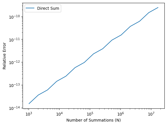

The Kahan summation algorithm is a method designed to minimize round-off errors during summation. By maintaining a separate compensation variable, it accounts for small errors that would otherwise be lost.

def Kahan_sum(x, n):
    c = 0.0 # compensation for lost low-order bits
    s = 0.0
    for i in range(n):
        xp = x - c # apply compensation
        c  = ((s + xp) - s) - xp # update compensation
        s += x - c # update sum
    return s

E_Kahan = [abs(Kahan_sum(x, n)/n - x) / x for n in N]

plt.loglog(N, E_simple, label='Simple Sum')
plt.loglog(N, E_Kahan,  label='Kahan Sum')
plt.xlabel('Number of Summations (N)')
plt.ylabel('Relative Error')
plt.legend()
plt.show() # optional in Jupyter Notebook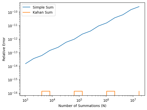

It is not recommended to write a for-loop in Python to sum numbers. Instead, numpy.sum() is usually a better choice. The numpy.sum() uses a more numerically accurate “partial pairwise summation” (see its documentation and source code). Here, we simply will try it out.

import numpy as np

def numpy_sum(x, n):
    X = np.repeat(x, n)
    return np.sum(X)

E_numpy = [abs(numpy_sum(x, n)/n - x) / x for n in N]

plt.loglog(N, E_simple, label='Simple Sum')
plt.loglog(N, E_Kahan,  label='Kahan Sum')
plt.loglog(N, E_numpy,  label='Numpy Sum')
plt.xlabel('Number of Summations (N)')
plt.ylabel('Relative Error')
plt.legend()
plt.show() # optional in Jupyter Notebook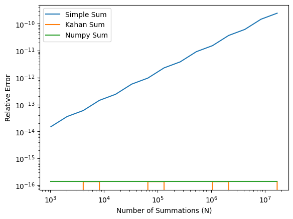

In the first homework, we will look into a concept called “catastrophic cancellation” and implement an algorithm that can handle it.

Catastrophic Cancellation¶

# HANDSON: run the above code here ...

We all learned in high school that the solutions (roots) to the qudratic equation $a x^2 + b x + c = 0$ is

\begin{align} x = \frac{-b \pm \sqrt{b^2 - 4 a c}}{2a}. \end{align}

(9)

Q: Why one of the roots become zero when solving the qudratic equation with $b = 1$ and $a = c = 10^{-9}$ ?

a = 1e-9
b = 1
c = 1e-9

x1 = (-b + (b*b - 4*a*c)**(1/2)) / (2*a)
x2 = (-b - (b*b - 4*a*c)**(1/2)) / (2*a)

print(f'{x1:.16f}, {x2:.16f}')

0.0000000000000000, -999999999.9999998807907104

It is straightforward to show in the limit $a, c \ll b$ , the roots are

\begin{align} x \approx -\frac{b}{a} \mbox{ or } -\frac{c}{b} \end{align}

(10)

Is it possible to recover the small root $-c/b$ ?

When $b > 0$ , a catastrophic cancellation (see below) happens only in the “+” equation. We may replace the first qudratic equation by its “conjugate” form

\begin{align} x = \frac{2c}{-b \mp \sqrt{b^2 - 4 a c}} \end{align}

(11)

Equivalently, we may use the “numerically stable form”,

\begin{align} x_1 &= \frac{-b - \mathrm{sign}(b)\sqrt{b^2 - 4 a c}}{2a} \\ x_2 &= \frac{c}{a x_1} \end{align}

(12)

as used by GSL and fadge.

Catastrophic cancellation occurs in numerical computing when subtracting two nearly equal numbers, leading to a significant loss of precision. This happens because the leading digits cancel out, leaving only less significant digits, which may already be corrupted by rounding errors in floating-point arithmetic. As a result, the final outcome can be far less accurate than expected.

For example, consider subtracting $x = 1.00000001$ and $y = 1.00000000$ . The exact result is 0.00000001, but if both numbers are rounded to six significant digits during storage (e.g., in single-precision floats), they might be stored as 1.00000. Subtracting these stored values yields 0, completely losing the small difference.

This issue is common in computations involving nearly equal terms, such as in numerical differentiation or solving linear systems, where precision errors can propagate. To mitigate catastrophic cancellation, techniques like reformulating equations to avoid such subtractions, using higher-precision arithmetic, or applying numerical methods specifically designed to reduce error can be employed.

Implementing a numerically stable form of the quadratic formula is left as a homework problem.

Other Floating Point¶

“Half percision” float16.
“Brain floating point” bfloat16, used for neural network.
long double, could be 80-bit or 128-bit, dependent on the system.

Encoding of Special Values¶

val    s_exponent_signcnd
+inf = 0_11111111_0000000
-inf = 1_11111111_0000000

val    s_exponent_signcnd
+NaN = 0_11111111_klmnopq
-NaN = 1_11111111_klmnopq

where at least one of k, l, m, n, o, p, or q is 1.

NaN Comparison Rules¶

In Python, like in C, the special value NaN (Not a Number) has unique comparison behavior. Any ordered comparison between a NaN and any other value, including another NaN, always evaluates to False.

To reliably check if a value is NaN, it is recommended to use the np.isnan() function from NumPy, as direct comparisons (e.g., x == np.nan) will not work as expected.

# Demonstrate NaN comparison rules

import numpy as np

x = np.nan
y = 1

print(x != x)
print(x >  x)
print(x <  x)
print(x >= x)
print(x <= x)
print(x == x)

print(x != y)
print(x >  y)
print(x <  y)
print(x >= y)
print(x <= y)
print(x == y)

True
False
False
False
False
False
True
False
False
False
False
False

Floating Point Exceptions¶

Q: What is the output of this simple code?

for e in range(1020, 1030):
    x = pow(2.0, e)
    print(f"2^{e} = {x}")

for e in range(-1070, -1080, -1):
    x = pow(2.0, e)
    print(f"2^{e} = {x:e}")

# HANDSON: try the above codes.

Abusing Floating Point Numbers: Fast Inverse Square Root

One fascinating example of taking advantage of floating-point representation is the fast inverse square root algorithm, famously used in computer graphics, particularly in the development of 3D engines like those in video games. This algorithm provides an efficient way to compute $1/\sqrt{x}$ , a common operation in tasks like normalizing vectors. Instead of relying on the standard floating-point math libraries, the algorithm “hacks” the floating-point representation by manipulating the bits directly to achieve a remarkably fast approximation of the result. This method takes advantage of how floating-point numbers are stored, using a clever combination of bitwise operations and mathematical magic to drastically speed up computation.

The following code is the fast inverse square root implementation from Quake III Arena, stripped of C preprocessor directives, but including modified comment text:

float Q_rsqrt( float number )
{
 	long i;
	float x2, y;
	const float threehalfs = 1.5F;

	x2 = number * 0.5F;
	y  = number;
	i  = * ( long * ) &y;                     // evil floating point bit level hacking
	i  = 0x5f3759df - ( i >> 1 );             // what the f**k?
	y  = * ( float * ) &i;
	y  = y * ( threehalfs - ( x2 * y * y ) ); // 1st iteration
//      y  = y * ( threehalfs - ( x2 * y * y ) ); // 2nd iteration, this can be removed

	return y;
}

ASTR 513

Overview

ASTR 513

Numerical Linear Algebra