
Welcome to ASTR 501!
This course is an introduction to computing for incoming astronomy and astrophysics graduate students. Course will cover basics of programming in Python and C/C++, including commonly-used libraries for astronomical research, an introduction to computer hardware including coprocessors such as GPUs, and some introductory concepts from computer science.
The course website is: https://
This course is recommended in conjunction with ASTR 513 Statistical and Computational Methods in Astrophysics, which meets every Monday and Wednesday 11am-12:15pm.
Also, every Thursday 2-3:30pm, we will have the weekly TAP Computation & Data Initiative meeting in SO N305. Please feel free to stop by as well.
Instructor and Contact Information
Instructor: Chi-kwan Chan
Email: chanc@arizona.edu (please include “ASTR 513” in subjects of emails)
Office: Steward Observatory N332
Office Hours: TBD
Instructor: Shuo Kong
Email: shuokong@arizona
Office: Steward Observatory N328
Office Hours: TBD
Scheduled Topics/Activities
| # | Week | Tuesday |
|---|---|---|
| 1 | Aug 24-Aug 30 | Jupyter Notebook and Python |
| 2 | Aug 31-Sep 6 | Unix/Linux, Shell, and Git |
| 3 | Sep 7-Sep 13 | Software Environment and Cloud Computing |
| 4 | Sep 14-Sep 20 | Make, Workflow, and GitHub Action |
| 5 | Sep 21-Sep 27 | C/C++ |
| 6 | Sep 28-Oct 4 | Code optimization |
| 7 | Oct 5-Oct 11 | Parallel Computing |
| 8 | Oct 12-Oct 18 | HPC and Slurm |
| 9 | Oct 19-Oct 25 | Hydrodynamic Simulation 1 |
| 10 | Oct 26-Nov 1 | Hydrodynamic Simulation 2 |
| 11 | Nov 2-Nov 8 | Hydrodynamic Simulation 3 |
| 12 | Nov 9-Nov 15 | No class (Veterans Day) |
| 13 | Nov 16-Nov 22 | Hydrodynamic Simulation 4 |
| 14 | Nov 23-Nov 29 | Presentation 1 |
| 15 | Nov 30-Dec 6 | Presentation 2 |
| 16 | Dec 7-Dec 13 | Visit UA HPC |
Grading Scale and Policies
This course provides pass/fail grades. Students who finish majority of hands-on labs and create reasonable projects would receive passing grades.
Usage of Generative AI
Homework, projects, and exams in this course are designed to help students apply class concepts, test their understanding, and develop skills in software development and scientific communication. Generative AI tools such as ChatGPT, Google Gemini, and GitHub Copilot can be valuable for brainstorming, exploring alternative approaches, clarifying confusing concepts, and debugging code. Students may also use these tools to clarify difficult concepts and to generate examples that aid their learning.
However, students must write their own code, take full responsibility for their work, and demonstrate a clear understanding of the underlying concepts. While AI tools can support learning, they may produce inaccurate, incomplete, or biased results. Students are responsible for verifying facts, testing code, and critically assessing all submitted material.
Any use of generative AI must be acknowledged or cited (see guidelines from UA library). Failure to disclose such use, or submitting work that is not original, will be considered a violation of academic integrity.
For questions, contact your instructor.
Introduction to Jupyter
The Jupyter Project provides tools, including Jupyter Notebook and JupyterLab, for interactive computing.
A Jupyter notebook is a single document that can mix together:
Code that you can run
Text explanations
Math equations
Data and plots
Images and interactive widgets
Think of it as a lab notebook that can explain an idea, run the
code, and show the results all in one place.
This form of programming is actually called “literate
programming”,
first introduced by in 1984 by Donald
Knuth, the creator of
TeX.
Proprietary programs like Mathematica and MATLAB have had similar notebook features for years. The difference is that Jupyter is open-source, built in Python, and freely available. This makes it one of the most popular tools in data science, astrophysics, and beyond.
How to Run This Notebook
These course materials (ASTR 501+513) are built using Jupyter Book, which combines Markdown files and Jupyter notebooks to provide lecture notes and hands-on labs. Because of this, each page can also be opened directly as a Jupyter notebook.
Jupyter notebooks can be used in many editors, including: VS Code (with Jupyter extensions) and Google Colab (runs in the cloud with no setup required).
To keep this first lab simple, we will use Google Colab.
Steps to open the notebook in Colab:
At the top right of this page, click the “Edit” pencil icon. This will open the notebook’s source page on GitHub.
On the GitHub page, find the “Open in Colab” badge near the top. Clicking this badge will open the notebook in Google Colab.
In Colab, run any code cell by either:
pressing “Shift + Enter”, or
clicking the ▶ Run button on the left of the cell.
With these steps, you can run Python code directly in your browser, without needing to install anything locally.
Markdown
In a Jupyter notebook (and hance Google Colab), there are mainly two types of cells.
By default, cells contain executable “Code”. Pressing “Shift + Enter” would run the code.
The cells that display documentation, such as this one, are “Markdown” cells. Pressing “Shift + Enter” would render the documentation.
Depending on which the Jupyter Lab Plugins you have, you may use basic markdown to write basic documentations or MyST to create fancy scientific paper.
Basic markdown syntax includes:
# A first-level heading
## A second-level heading
### A third-level heading
**bold text** or __bold text__
*italic* or _italic_
> Text that is a quote
[A link](URL)
HANDSON:
Turn this cell into a markdown cell.
Write a short introduction about yourself and your research interest.
Try different formatting methods.
* Can you display equations?
* Can you use non-ASCII characters, e.g., emoji?
* Why does CK always add a newline after a period?
* Why does CK always break a long sentence?
An Introduction to Python
Python is a high-level programming language created in the late 1980s by Guido van Rossum. It was first released in 1991 with the goal of being both powerful and easy to read. Its name comes from Monty Python’s Flying Circus (not from the snake).
Today, Python is one of the most widely used programming languages in the world. It is especially popular in data science, artificial intelligence, and scientific computing, largely because:
The syntax is simple and readable, making it beginner-friendly.
It has a vast ecosystem of libraries (e.g., NumPy, SciPy, pandas, matplotlib, scikit-learn, TensorFlow, PyTorch).
It supports both quick prototyping and large-scale applications.
It is open-source and has a strong worldwide community.
It even has a documentary now!!!
In astrophysics and many other sciences, Python has become the standard language for data analysis, modeling, and visualization.
Python code can be written and executed interactively in Jupyter notebooks. In fact, the name “Jupyter” comes from the three programming langauge Julia, Python, and R. Let’s begin with the basics.
You may skip this if you already know Python.
1. Printing
Use the print() function to display output.
# Example: Print a message

print("Hello, world!  Welcome to ASTR 501!")
Hello, world! Welcome to ASTR 501!
# HANDSON: Change the message

print("Your custom message here")
Your custom message here
# HANDSON: What happen if you just type a message without print?
# HANDSON: Instead of print(), try to use display().
#          Do you know what is the difference?
2. Variables and Data Types
Python supports various data types such as integers, floats, strings, and booleans.
# Example: variable assignment with different types

i       = 1           # Integer
j       = 2**345      # Integers have arbitrary precision
x       = 3.14        # Float
y       = 4e6         # Float in scientific notation
z       = 5 + 6j      # Complex number
astr    = "Astronomy" # String
is_cool = True        # Boolean

print("i =", i)
print("j =", j)
print("x =", x)
print("y =", y)
print("z =", z)
print("astr =", astr)
print("is_cool =", is_cool)
i = 1
j = 71671831749689734737838152978190216899892655911508785116799651230841339877765150252188079784691427704832
x = 3.14
y = 4000000.0
z = (5+6j)
astr = Astronomy
is_cool = True
# HANDSON: Define and print variables

year       = ...
height     = ...
name       = ...
is_student = ...

print("Year:", year)
print("Height:", height)
print("Name:", name)
print("Is student:", is_student)
3. Basic Arithmetic
Python can handle basic mathematical operations.
# Examples of arithmetic

addition       = 1 + 1
subtraction    = 2 - 1
multiplication = 3 * 4
division       = 5 / 2 # this is called "truediv"
division2      = 5 //2 # this is called "floordiv"
remainder      = 5 % 2 # this is called "mod"
power          = 5 **2

print("Addition:",       addition)
print("Subtraction:",    subtraction)
print("Multiplication:", multiplication)
print("Division:",       division)
print("Division2:",      division2)
print("Remainder:",      remainder)
print("Power:",          power)
Addition: 2
Subtraction: 1
Multiplication: 12
Division: 2.5
Division2: 2
Remainder: 1
Power: 25
# HANDSON: test out true division `/`, floor division `//`, and "mod"
#          `%` with different combinations of integers and floating
#          point numbers.
#          Do the results make sense?
#          Can you provide an equation that summarizes the logic of
#          these operators?
4. Lists
Lists are ordered collections of items.
# Example: Creating a list
numbers = [1, 2, 3, 4, 5]
print("Original list:", numbers)

# Accessing elements
print("First element:", numbers[0])
print("Last element:", numbers[-1])

# Adding elements
numbers.append(6)
print("List after appending:", numbers)

# Removing last elements
numbers.pop()
print("List after removing last element:", numbers)

# Removing specific elements
numbers.remove(i) # note that `i` was defined above
print("List after removing", i, ":", numbers)
Original list: [1, 2, 3, 4, 5]
First element: 1
Last element: 5
List after appending: [1, 2, 3, 4, 5, 6]
List after removing last element: [1, 2, 3, 4, 5]
List after removing 1 : [2, 3, 4, 5]
# HANDSON: create your own list and manipulate it.

# Create a list
fruits = ...
print("Fruits:", fruits)

# Add an element to the list
...
print("Fruits:", fruits)

# Remove an item
...
print("Fruits:", fruits)
# HANDSON: lists also support operators.
# Try using `+` and `*` on lists.
# What do you get?
# HANDSON: Python has a data structure very similar to list
#          called `tuple`.
#          The syntax to create it is `t = (1, 2, 3, ...)`.
#          Create a tuple and compare it with a list.
#          What's the difference?
5. For Loops
Loops allow you to iterate over a sequence of items.
# Example: Loop through a list

for number in numbers:
    print("Number:", number)
Number: 2
Number: 3
Number: 4
Number: 5
# Example: Use an iterable instead of a list
for number in range(10):
print("Number:", number)Number: 0
Number: 1
Number: 2
Number: 3
Number: 4
Number: 5
Number: 6
Number: 7
Number: 8
Number: 9
# HANDSON: Write a loop to print squares of numbers.
#          Note that we use something called a "formatted string",
#          or "f-strings", here.

...
    print(f"Square of {i} is {i ** 2}")
6. Functions
Functions allow you to reuse code.
# Example: Define a function
def greet(name):
    return f"Hello, {name}!  Welcome to ASTR 501!"

# Call the function
message = greet(name)
print(message)
# HANDSON: Function to calculate circle area
def circle_area(radius):
...
# Test the function
area = circle_area(5)
print("Area of circle with radius 5:", area)7. NumPy: Numerical Computing
Python’s power comes from its libraries.
For scientific computing, numpy and matplotlib are probably the
two most important libraries.
Let’s explore their capabilities.
NumPy provides support for large multi-dimensional arrays and matrices, along with mathematical functions to operate on them.
# Example: Using NumPy
import numpy as np

# Create an array
array = np.array([1, 2, 3, 4, 5])
print("Array:", array)

# Perform operations
squared = array ** 2
print("Squared Array:", squared)

# Generate a range of numbers
linspace = np.linspace(0, 10, 11)
print("Linspace:", linspace)
Array: [1 2 3 4 5]
Squared Array: [ 1 4 9 16 25]
Linspace: [ 0. 1. 2. 3. 4. 5. 6. 7. 8. 9. 10.]
NumPy’s core functions are written in C (see, e.g., here). Using NumPy for large arrays is much faster than for loop in python.
array = range(10_000) # you may add underscore to integers to improve readibility.%%time
# `%%time` is a "magic command" of IPython.
# it prints the wall time for the entire cell.
squared = []
for a in array:
squared.append(a*a)CPU times: user 1.83 ms, sys: 136 μs, total: 1.97 ms
Wall time: 1.98 ms
array = np.arange(10_000)%%time
squared = array * arrayCPU times: user 171 μs, sys: 17 μs, total: 188 μs
Wall time: 183 μs
# HANDSON: NumPy calculations

# Create an array of numbers from 1 to 10
numbers = ...

# Calculate their squares and square roots
squares = ...
roots   = ...

print("Numbers:", numbers)
print("Squares:", squares)
print("Square Roots:", roots)
8. Matplotlib: Data Visualization
Matplotlib is a plotting library for creating static, animated, and interactive visualizations.
# Example: Plotting with Matplotlib
import matplotlib.pyplot as plt

# Create data with NumPy
x = np.linspace(0, 10, 100)
y = np.sin(x)

# Create a plot with Matplotlib
plt.plot(x, y, '-o', label='sin(x)')
plt.title("Sine Wave")
plt.xlabel("x")
plt.ylabel("sin(x)")
plt.legend()
plt.grid()

# Show and save figure
plt.show()  # optional in jupyter notebook
plt.savefig('sin.pdf')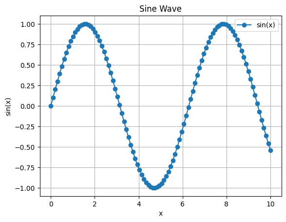
<Figure size 640x480 with 0 Axes># HANDSON: Create a plot
# Let's try to plot two curves in a single plot
x = np.linspace(0, 2 * np.pi, 100)
y1 = np.sin(x)
y2 = np.cos(x)
# Plot both sine and cosine
...
...
# Customize the plot
...
# Show and save figure
...Clearly this does not cover all important python topics.
Specifically, we left out dictionary, set, condition statements
such as if-elif-else, etc.
But hopefully these are enough for you to get started in ASTR 501+513.
As the semester goes, we will pick up more python.
Slightly More Advanced Python
If you already know the basics of Python, instead of getting bored, let’s get into slightly more advanced topics. Specifically, let’s explore NumPy, one of the most important libraries for scientific computing. NumPy provides:
High-performance multi-dimensional arrays (the
ndarray)Concise syntax for numerical operations
Speed-ups over pure Python, since many operations run in optimized C code
In astrophysics and data science, NumPy is a foundation for almost every other scientific library (such as SciPy and AstroPy).
Array Creation and Slicing
NumPy arrays look similar to Python lists, but are much faster and more powerful.
import numpy as np

a = np.arange(10)   # array with values 0 to 9
print(a)

# Slicing: extract parts of the array
print(a[2:7])       # elements 2 through 6
print(a[:5])        # first 5 elements
print(a[::2])       # every other element
[0 1 2 3 4 5 6 7 8 9]
[2 3 4 5 6]
[0 1 2 3 4]
[0 2 4 6 8]
a = np.random.normal(size=(5,4))  # 5x4 random array
print(a)

# Slicing: selecting rows
print(a[1:3])       # rows 1 through 3
print(a[:2])        # first 2 rows
print(a[::2])       # every other row

# Slicing: selecting columns
print(a[:,1:3])       # columns 1 through 3
print(a[:,:2])        # first 2 columns
print(a[:,::2])       # every other columns
[[ 1.21695026 0.93138844 -0.84416748 1.53668701]
[-0.98623524 -0.66784365 1.51820536 0.24356732]
[ 0.88424021 -0.32613532 -0.69095756 -0.81037232]
[ 2.91239298 1.30947663 1.80968095 -0.08263627]
[-0.27998714 0.65708405 0.08281572 1.76169808]]
[[-0.98623524 -0.66784365 1.51820536 0.24356732]
[ 0.88424021 -0.32613532 -0.69095756 -0.81037232]]
[[ 1.21695026 0.93138844 -0.84416748 1.53668701]
[-0.98623524 -0.66784365 1.51820536 0.24356732]]
[[ 1.21695026 0.93138844 -0.84416748 1.53668701]
[ 0.88424021 -0.32613532 -0.69095756 -0.81037232]
[-0.27998714 0.65708405 0.08281572 1.76169808]]
[[ 0.93138844 -0.84416748]
[-0.66784365 1.51820536]
[-0.32613532 -0.69095756]
[ 1.30947663 1.80968095]
[ 0.65708405 0.08281572]]
[[ 1.21695026 0.93138844]
[-0.98623524 -0.66784365]
[ 0.88424021 -0.32613532]
[ 2.91239298 1.30947663]
[-0.27998714 0.65708405]]
[[ 1.21695026 -0.84416748]
[-0.98623524 1.51820536]
[ 0.88424021 -0.69095756]
[ 2.91239298 1.80968095]
[-0.27998714 0.08281572]]
# HANDSON: In python, negative indices are valid.
#          Try to use negative indices to access and slice
#          numpy arrays.
#          Does the result match your expectation?
Broadcasting
Broadcasting allows NumPy to apply operations on arrays of different shapes without writing explicit loops.
# EXAMPLE: adding vector and scalar

X = np.array([1, 2, 3])
Y = np.array([10])

print(X + Y)   # Y is automatically "broadcast" to match X
[11 12 13]
# EXAMPLE: adding column and row vectors, i.e., "outer sum"

X = np.arange(3).reshape(3,1)  # column vector
Y = np.arange(3)               # row vector

print("X =\n", X)
print("Y =",   Y)
print("X + Y =\n", X + Y)      # produces a 3x3 matrix
X =
[[0]
[1]
[2]]
Y = [0 1 2]
X + Y =
[[0 1 2]
[1 2 3]
[2 3 4]]
# EXAMPLE: use `np.newaxis` for "outer sum"

X = np.arange(3)  # row vector
Y = np.arange(3)  # row vector

print("X =\n", X)
print("Y =",   Y)
print("X + Y =\n", X[:,np.newaxis] + Y)  # produces a 3x3 matrix
X =
[0 1 2]
Y = [0 1 2]
X + Y =
[[0 1 2]
[1 2 3]
[2 3 4]]
# EXAMPLE: scaling columns of a matrix

M = np.arange(12).reshape(3, 4)
V = np.array([1, 10, 100, 1000])   # 1D array with 4 elements

print("M =\n", M)
print("M * V =\n", M * V)  # V is broadcast across rows
M =
[[ 0 1 2 3]
[ 4 5 6 7]
[ 8 9 10 11]]
M * V =
[[ 0 10 200 3000]
[ 4 50 600 7000]
[ 8 90 1000 11000]]
# EXAMPLE: pairwise distances (without loops)

P = np.array([[0, 0], [1, 0], [0, 1]])

# Broadcasting to compute squared distances
D = P[:, np.newaxis, :] - P[np.newaxis, :, :]
DD = np.sum(D**2, axis=-1)

print(DD)
[[0 1 1]
[1 0 2]
[1 2 0]]
# EXAMPLE: normalizing vectors

V = np.array([[3, 4], [1, 1], [0, 5]])

L = np.sqrt(np.sum(V**2, axis=1))   # shape (3,)
N = V / L[:, np.newaxis]       # broadcast to (3,2)

print(N)
[[0.6 0.8 ]
[0.70710678 0.70710678]
[0. 1. ]]
# HANDSON: try to use both reshape() and newaxis to
#          implement outer product of two vectors.
Einstein Summation (einsum)
The einsum() function gives a compact way to express many linear algebra
operations using Einstein summation notation.
# Dot product of two vectors
X = np.array([1, 2, 3])
Y = np.array([4, 5, 6])
print(np.einsum('i,i->', X, Y))

# Matrix multiplication
A = np.arange(9).reshape(3, 3)
B = np.arange(9, 18).reshape(3, 3)
print(np.einsum('ik,kj->ij', A, B))

# Summing over axes
print(np.einsum('ij->i', A))  # row sums
print(np.einsum('ij->j', A))  # column sums
32
[[ 42 45 48]
[150 162 174]
[258 279 300]]
[ 3 12 21]
[ 9 12 15]
# HANDSON: try to use einsum() to
#          implement outer product of two vectors.
Meshgrid and Vector Fields
We can use np.meshgrid() to build 2D grids.
It is useful for plotting vector fields.
import matplotlib.pyplot as plt

x = np.linspace(-2, 2, 20)
y = np.linspace(-2, 2, 20)
X, Y = np.meshgrid(x, y)

U = -Y   # vector field component in x
V =  X   # vector field component in y

plt.figure(figsize=(5,5))
plt.quiver(X, Y, U, V)
plt.xlabel("x")
plt.ylabel("y")
plt.title("Vector Field: Rotation Around Origin")
plt.axis("equal")
plt.show()  # optional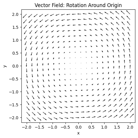
# HANDSON: try to use einsum() to compute the norm of the vector field
#          and over (under?) plot it as a "heatmap" with the vector field.
#          What is the advantage (or disadvantage) to use einsum() compared
#          to simple numpy operations?
Summary
In this lab, you learned:
The basic of Jupyter Notebook
The basic of Python:
How to print output
Variables and data types
Basic arithmetic operations
Working with lists
Using loops
Writing functions
Introduction to NumPy for numerical computations
Introduction to Matplotlib for data visualization
Slightly more advanced Python:
Array Creation and Slicing
Broadcasting
Einstein Summation
Meshgrid